The model maps

GIS files to build the model and for reporting

2023-02-03

Bangladesh

 

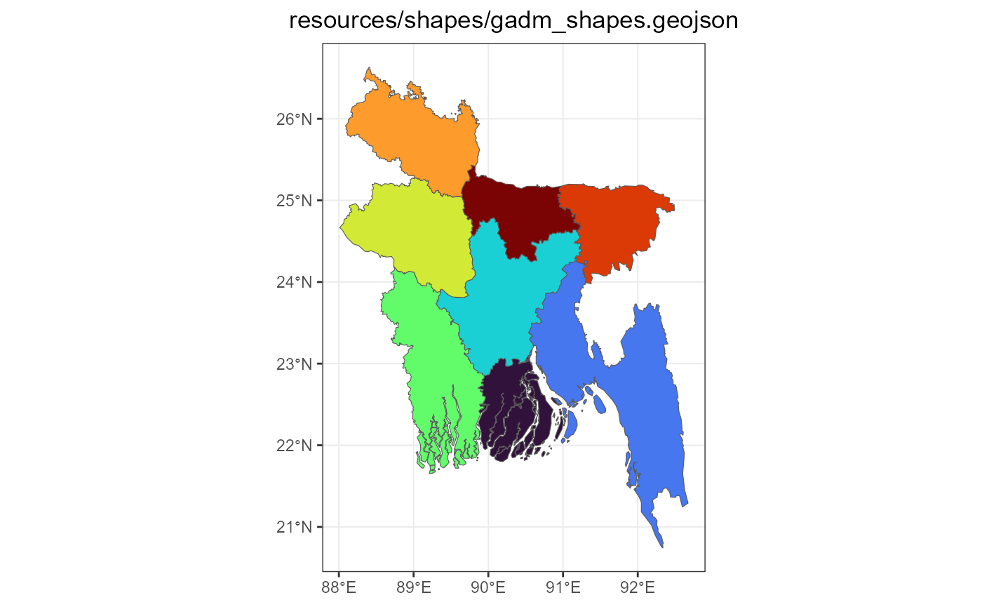
GDAM map (administrative regions)

ttl <- paste0(gis$adm1$sf$COUNTRY[1], " (", gis$adm1$sf$GID_0[1], "), ", 
               nrow(gis$adm1$sf), " regions")

show_legend <- nrow(gis$adm1$sf) <= 30

ggplot(gis$adm1$sf) +
  geom_sf(aes(fill = NAME_1), show.legend = show_legend) + 
  scale_fill_viridis_d(option = "H", name = "") +
  labs(title = ttl) +
  rev_theme_map()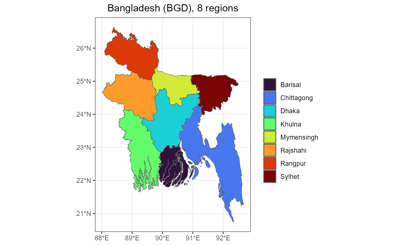

code

## Basic plots of `sp` and `sf`
# sf
plot(gis$adm1$sf[1], main = ttl, key.pos = 1)
length(gis$adm1$sp) # number of regions

# sp
plot(gis$adm1$sp, col = rainbow(11), axes = T, border = rgb(1,1,1,0.2), main = ttl)

Maps from PyPSA-Earth model dataset

pypsa_geojson <- rev_list_files(p$pypsa$dir, search.pattern = ".geojson$")
# pypsa_geojson
gis_pypsa <- rev_list_files(p$pypsa$dir, search.pattern = ".geojson$", 
                            fun = st_read)
object.size(gis_pypsa)
# gis$pypsa <- gis_pypsa
# save(file.path(p$dir$data, "gis_pypsa.RData"))

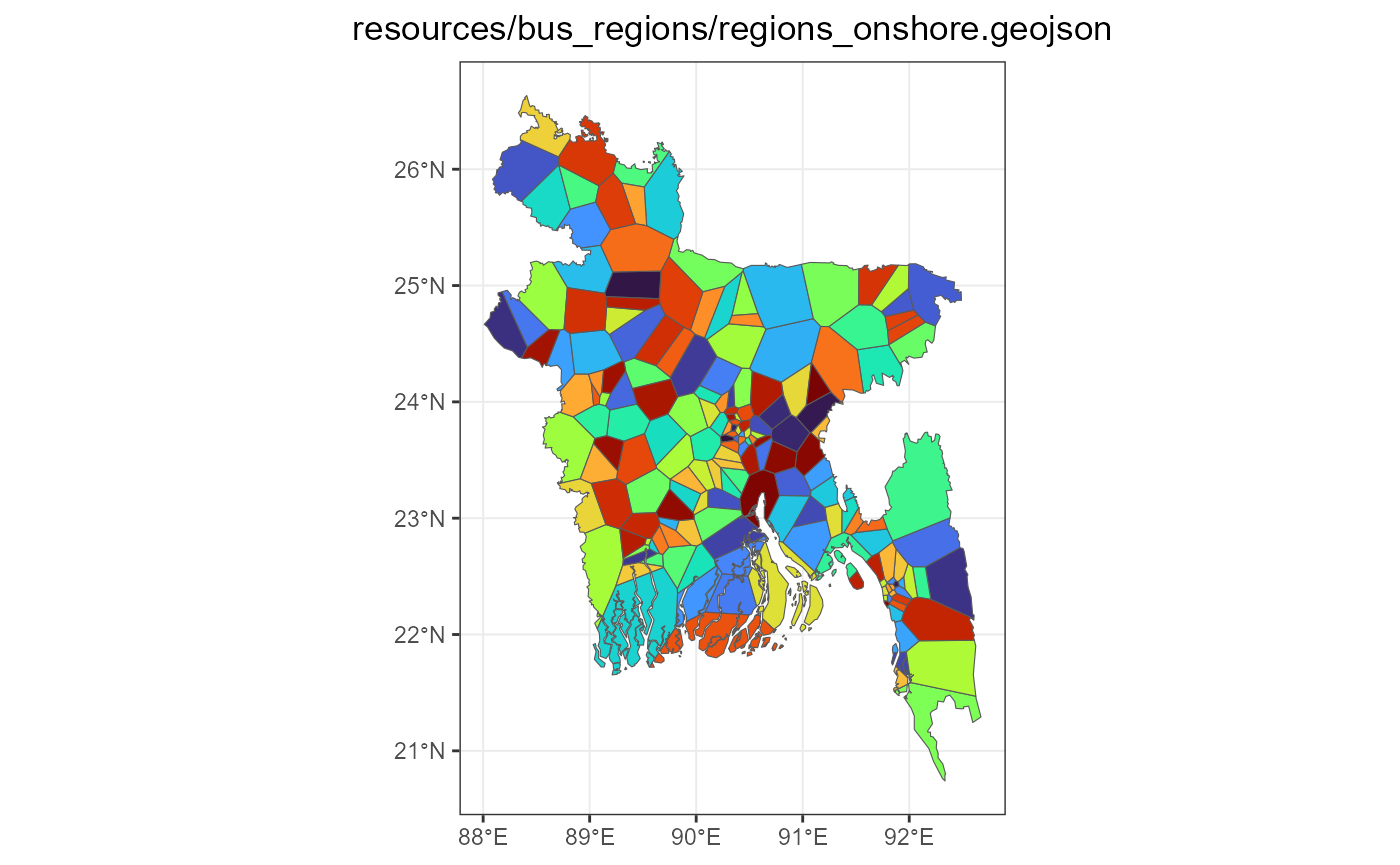
gis_onshore <- rev_list_files(
  p$pypsa$dir, search.pattern = "regions_onshore_elec_s_[0-9]+.geojson$", 
  fun = st_read) %>% rev_unlist(level = 100)
gis_onshore <- gis_onshore[[1]]

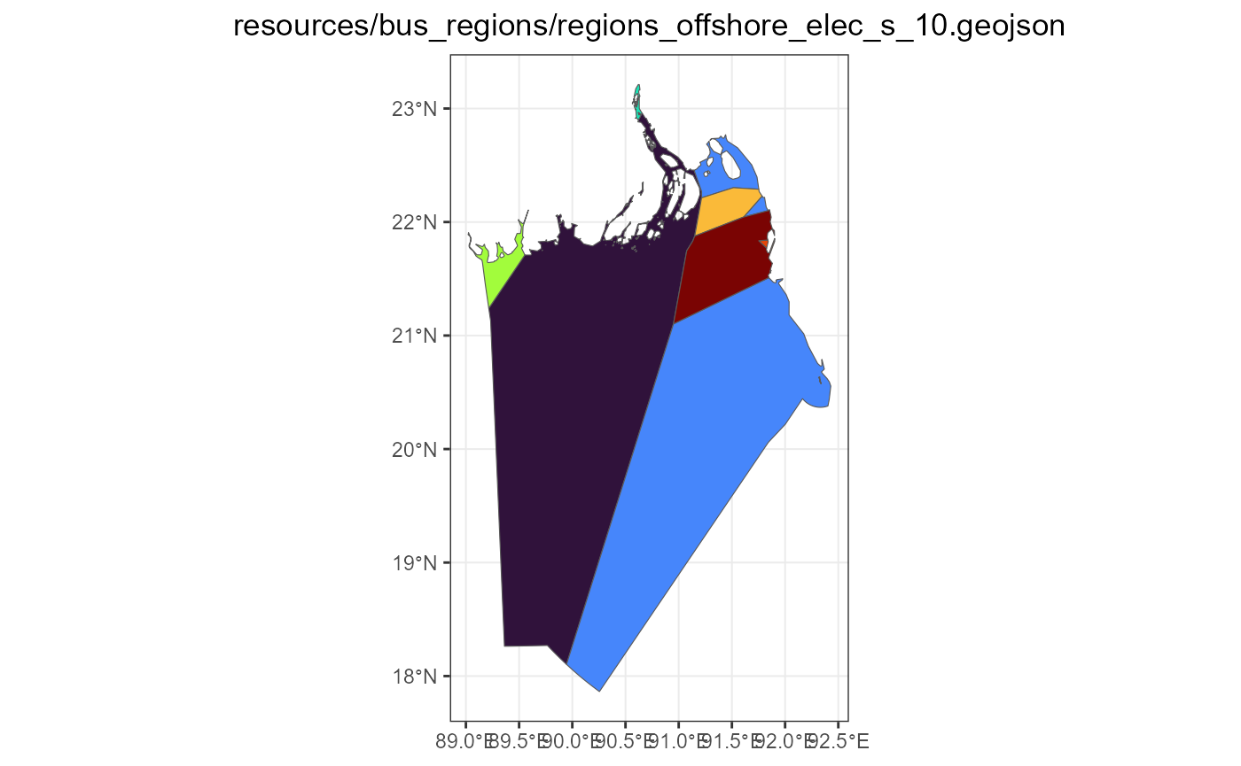
gis_offshore <- rev_list_files(
  p$pypsa$dir, search.pattern = "regions_offshore_elec_s_[0-9]+.geojson$", 
  fun = st_read) %>% rev_unlist(level = 10)
gis_offshore <- gis_offshore[[1]]

The current model map

# world map (for background)
worldmap <- rnaturalearth::ne_countries(
  scale = 'medium', type = 'map_units', returnclass = 'sf')

xy_on <- st_bbox(gis_onshore); xy_off <- st_bbox(gis_offshore)

ggplot() +
  geom_sf(data = worldmap) +
  geom_sf(
    aes(fill = name), color = "black", 
    show.legend = if_else(nrow(gis_onshore) <= 50, TRUE, FALSE),
    data = gis_onshore) +
  geom_sf(
    aes(fill = name),alpha = .5,
    show.legend = if_else(nrow(gis_onshore) <= 50, TRUE, FALSE),
    data = gis_offshore) +
  coord_sf(xlim = c(min(xy_on["xmin"], xy_off["xmin"]), 
                    max(xy_on["xmax"], xy_off["xmax"])),
           ylim = c(min(xy_on["ymin"], xy_off["ymin"]), 
                    max(xy_on["ymax"], xy_off["ymax"]))) +
  labs(title = paste0(gis$adm1$sf$COUNTRY[1], 
                      " (", gis$adm1$sf$GID_0[1], "), ",
                      "onshore and offshore clusters")) +
  theme_bw()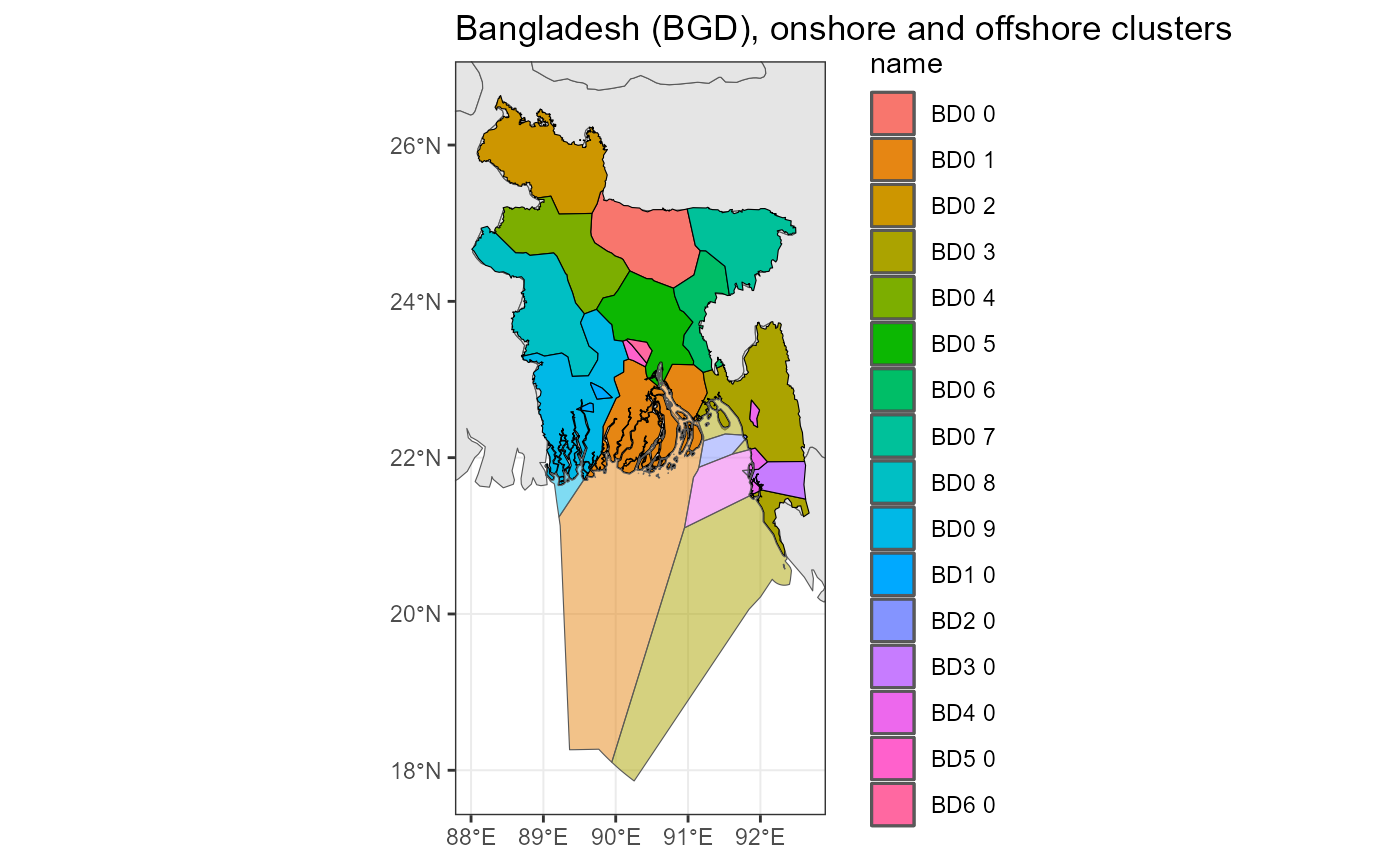

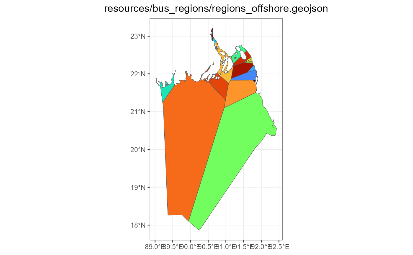
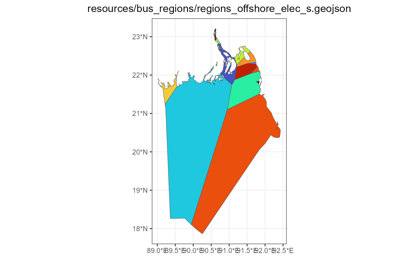
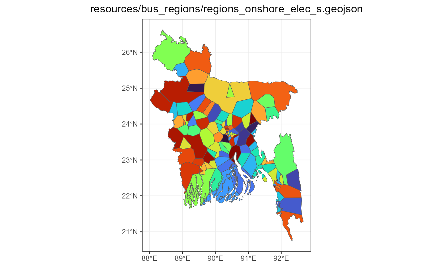
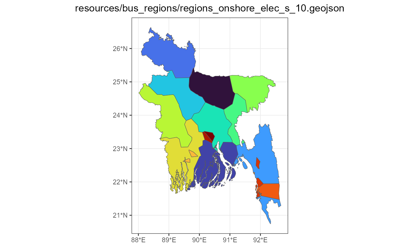
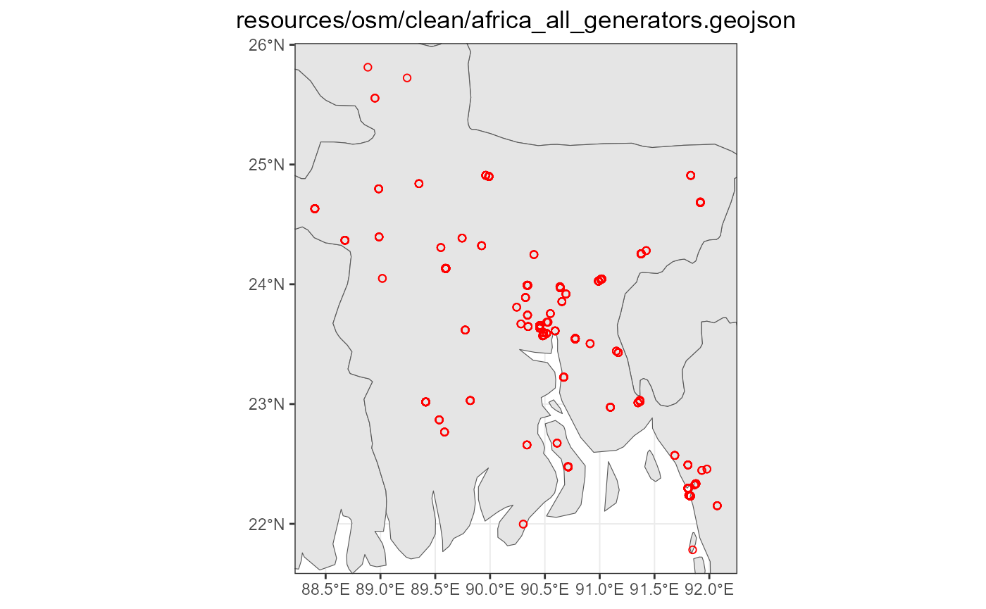
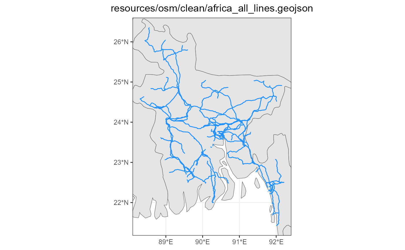
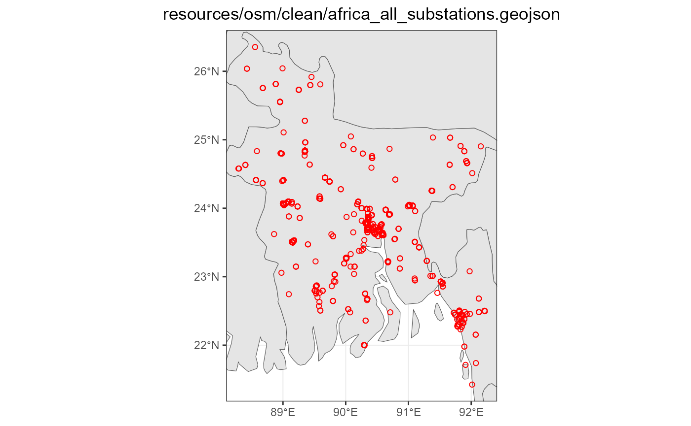
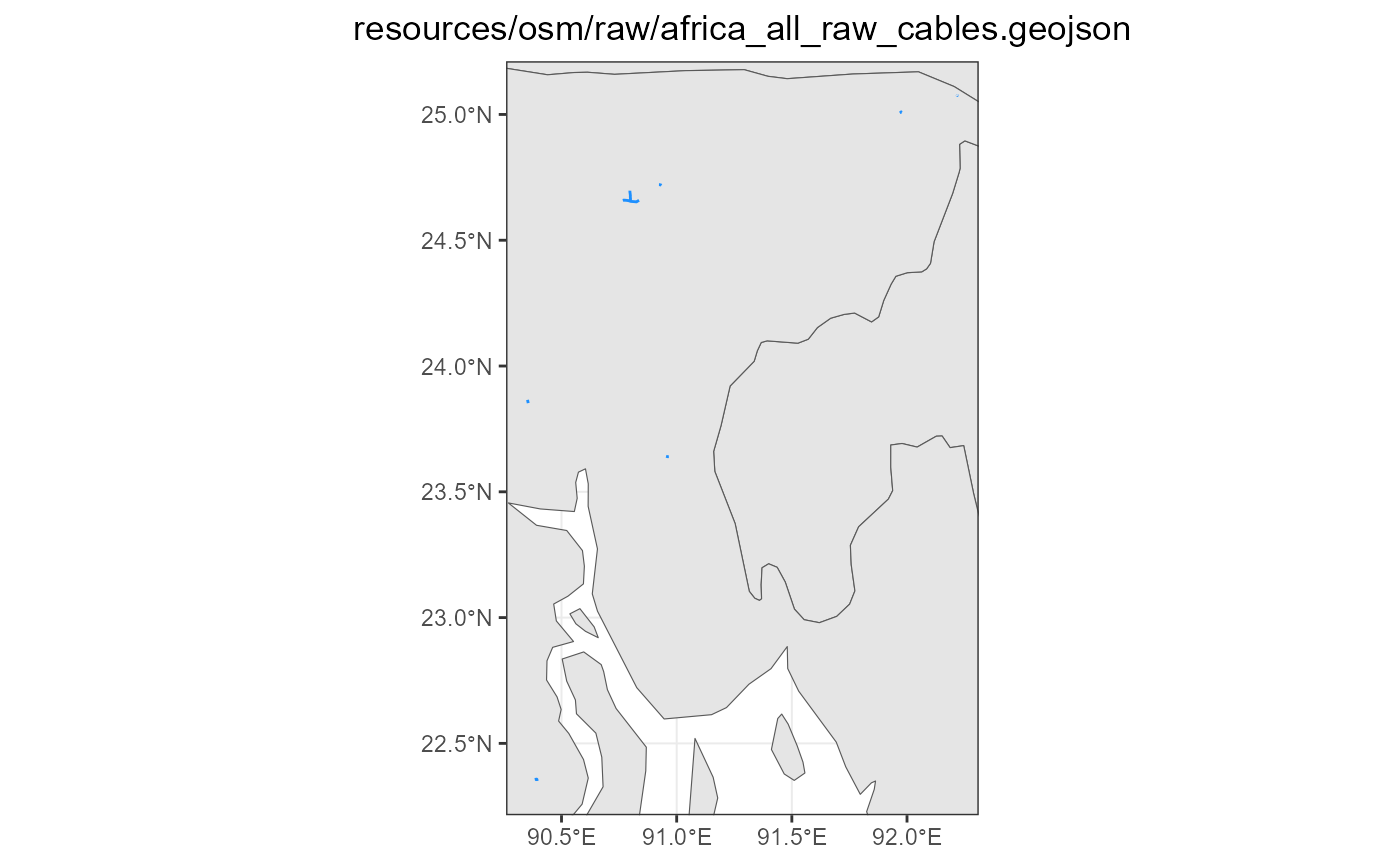
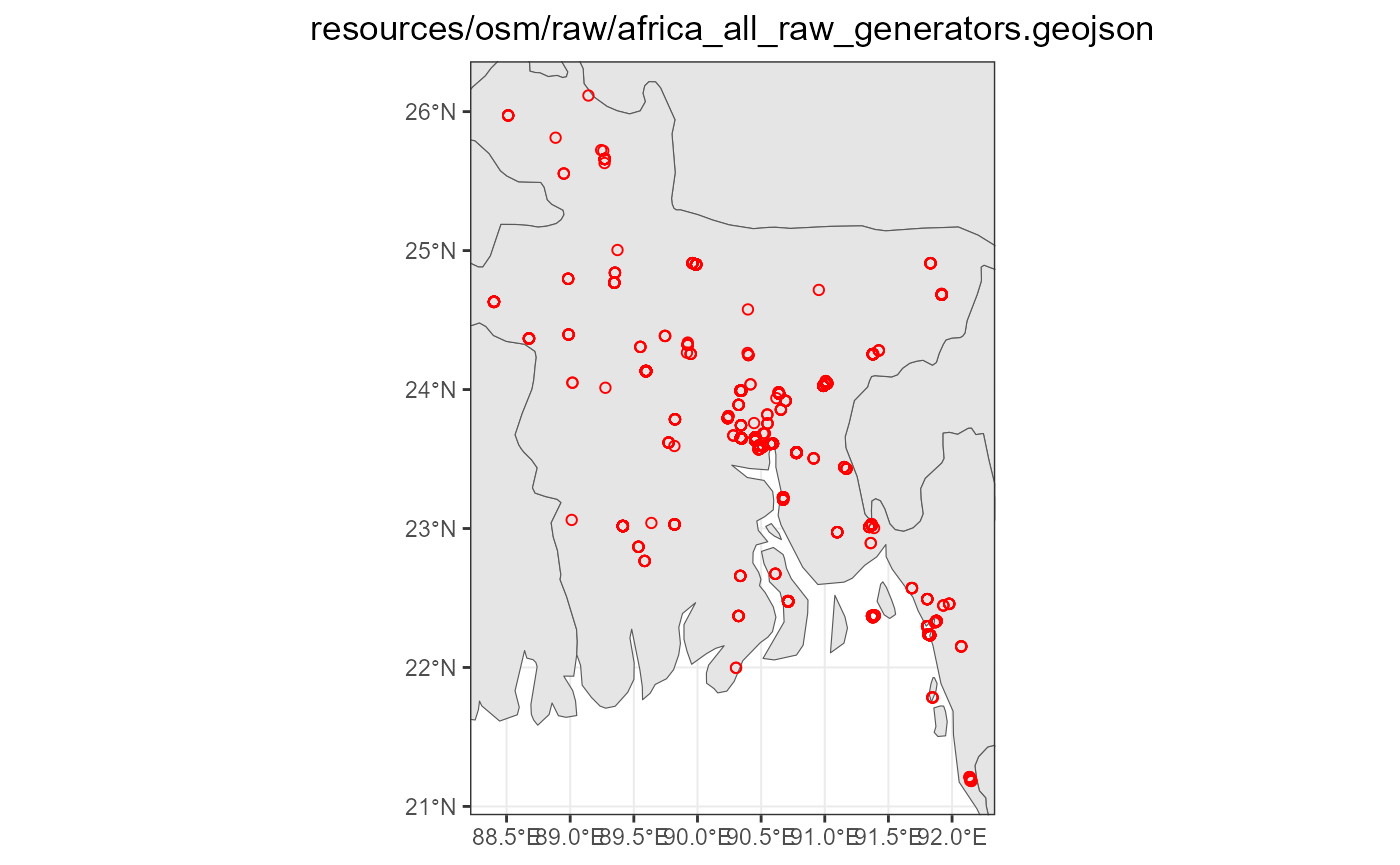
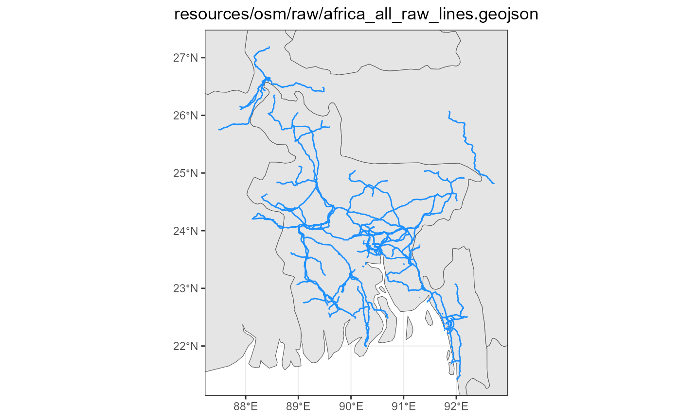
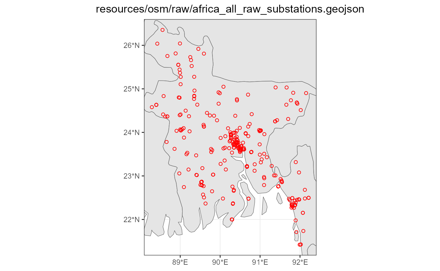
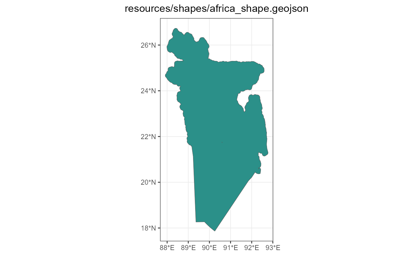
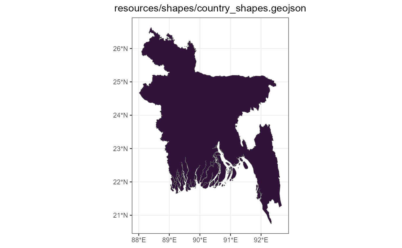
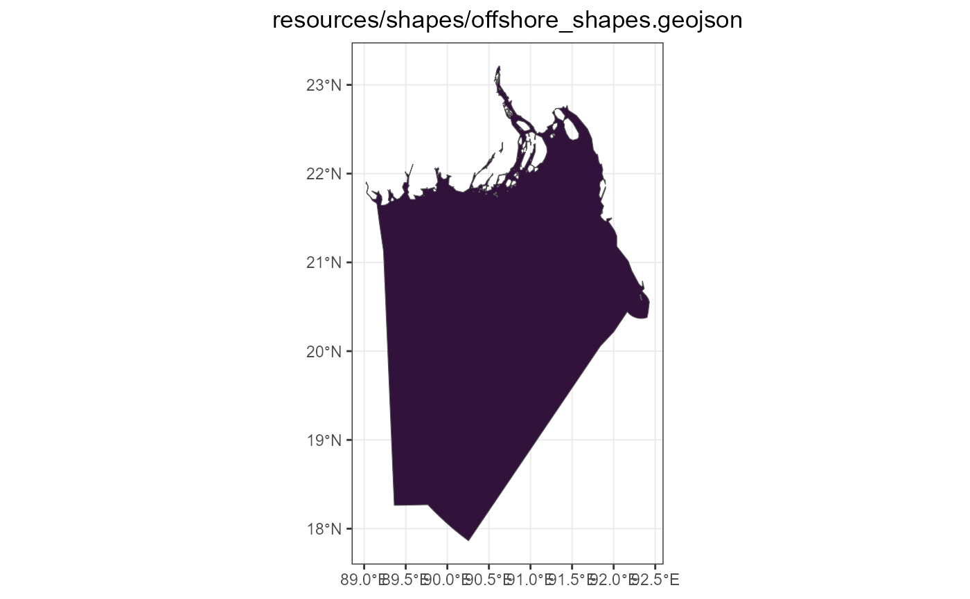
All existing maps

gis_pypsa <- gis_pypsa %>% rev_unlist(level = 5)

for (i in 1:length(gis_pypsa)) {
  g <- gis_pypsa[[i]]
  ii <- sapply(st_drop_geometry(g), function(x) length(unique(x))) == nrow(g)
  ii <- which(ii)[1]
  nm <- names(gis_pypsa)[i]
  if (any(grepl("POINT", class(st_geometry(g))))) {
    a <- ggplot(g) +
      geom_sf(data = worldmap) +
      geom_sf(color = "red", show.legend = FALSE, shape = 1) +
      labs(title = nm) +
      coord_sf(xlim = st_bbox(g)[c(1,3)], ylim = st_bbox(g)[c(2,4)]) +
      # scale_fill_viridis_d(option = "H") +
      theme_bw()
  } else if (any(grepl("LINE", class(st_geometry(g))))) {
    a <- ggplot(g) +
      geom_sf(data = worldmap) +
      geom_sf(color = "dodgerblue", show.legend = FALSE) +
      labs(title = nm) +
      coord_sf(xlim = st_bbox(g)[c(1,3)], ylim = st_bbox(g)[c(2,4)]) +
      # scale_fill_viridis_d(option = "H") +
      theme_bw()
  } else {
    a <- ggplot(g) +
      geom_sf(aes(fill = .data[[names(g)[ii]]]), show.legend = FALSE) +
      labs(title = nm) +
      theme_bw()
    if (is.numeric(g[[ii]])) {
      a <- a + scale_fill_viridis_c(option = "D")
    } else {
      a <- a + scale_fill_viridis_d(option = "H")
    }
  }
  a <- a + theme(plot.title = element_text(hjust = 0.5))
  print(a)
}