Import PyPSA-Earth model

and build Switch and energyRt models

2023-02-03

 

[WORK IN PROGRESS]

  This documented is a reproducible example of “translation” of PyPSA-Earth electric power sector models to Switch and energyRt models. The three models have differences in representation of generating technologies, energy storage, and other model elements. Notes along the script with an interim output describe all steps of the process of the “translation”, e.g. remapping the data and parameters from PyPSA to Switch and energyRt, and describes the structure of the model and the data. This experimental exercise has a goal to compare and analyze structural differences between the three models.
The script in this document reads Yaml configuration file for a country which sets input directories (with PyPSA-Earth files) and destination directories for raw csv files of the data-sets, Switch and/or energyRt models. There are two ways to run script in the vignette for a country for which PyPSA-Earth dataset is available. First, it can be downloaded to your project’s home directory and “knitted” in RStudio (see “Knit” menu for “.rmd” files). In this case edit the vignette’s YAML-header if necessary (top of the file). Alternatively, the whole script can be executed from a R-console (see Get started.)

Bangladesh model

Setup

Load required libraries, set country by iso3c code for the evaluation, read yaml file, and load maps.

library(tidyverse)
library(ggrepel)
library(sf)
library(sp)
library(data.table)
library(revaluation)
library(energyRt)

# Set the country
rev_set_country(params$iso3c)
#> Country code set to 'BGD' (Bangladesh)
rev_country()
#> [1] "BGD"

# read configuration file for the country
p <- rev_read_yaml(path = params$yaml_path)
#> "data/BGD" already exists
#> "scenarios/BGD" already exists
#> "tmp/BGD" already exists
#> "tmp/shared/BGD" already exists

# load maps
(load(p$gis_file))
#> [1] "gis"

Import PyPSA-Earth dataset

Read PyPSA’s .nc file with the model input data, group by sets, and return as a list with tables. Every table is matched with known set of parameters (column names) for further use in the “translation” process to other models.

# read data from pypsa network nc-file (see config_{}.yml file)
nc <- rev_read_pypsa_nc(p$pypsa$files$network)
#> Reading: I:/odpp/pypsa/world_mod_data/BD/networks/elec_s_10_ec_lcopt_Co2L-1H.nc
#> nc-file dimensions -> table name
#> D13,D0 -> generators_cf
#> D4,D0 -> storage_inflow
#> D6,D0 -> loads
#> D10 -> stores
#> D11 -> lines
#> D12 -> generators
#> D13 -> generators_cf_set
#> D0 -> snapshots
#> D1 -> unrecognized - no matches
#> D2 -> global_constraints
#> D3 -> storage_units - guessed
#> D4 -> storage_units_set
#> D5 -> loads_map
#> D6 -> loads_set
#> D7 -> buses
#> D8 -> carriers
#> D9 -> links
class(nc) # tables stored in the named list (use `names(nc)` to print names)
#> [1] "list"

Export to .csv

Optional (see save_csv parameter in Yaml header of the vignette) saving of the tables as .csv files to the given in yaml file directory.

# set directory for csv files ('csv_dir') and execute the chunk
csv_dir <- file.path(p$switch$dir, "pypsa/raw")
dir.create(csv_dir, showWarnings = F, recursive = T)
message("Saving raw csv files: ", csv_dir)

for (i in 1:length(nc)) {
  if (is.data.frame(nc[[i]])) {
    fname <- file.path(csv_dir, paste0(names(nc)[i], ".csv"))
    cat(fname, "\n")
    fwrite(nc[[i]], fname, row.names = F)
  }
}

Mapping functions for sets/names

Conventions:
…

if (F) { # (optional)
# Edit and re-load this function to change mapping or names
  rev_bus2reg <- function(x, num_width = 2, sep = "", map = NULL) {
    # browser()
    NN <- str_extract(x, "[0-9]+$")
    TXT <- str_replace(x, NN, "") %>% str_trim() %>% toupper()
    if (any(grepl("[0-9]", TXT)))
      stop("Unrecognized (non-ending or multiple) numeric indexes in names")
    NN <- formatC(as.integer(NN), width = num_width, flag = "0", format = "d")
    paste(TXT, NN, sep = sep)
  }
}

if (F) { # (optional)
  # Edit and load this function to change mapping or names
  # details: ?carriers2comm
carriers2comm <- function(x) {
  # mapping carriers to commodities
  x <- toupper(x)
  x[grepl("COA", x, ignore.case = TRUE)] <- "COA"
  x[grepl("OIL", x, ignore.case = TRUE)] <- "OIL"
  x[grepl("CGT", x, ignore.case = TRUE)] <- "GAS"
  x[grepl("WIND", x, ignore.case = TRUE)] <- "WIN"
  x[grepl("SOLAR", x, ignore.case = TRUE)] <- "SOL"
  x[grepl("LIGN", x, ignore.case = TRUE)] <- "LIG"
  x[grepl("BIO", x, ignore.case = TRUE)] <- "BIO"
  x[grepl("NUC", x, ignore.case = TRUE)] <- "NUC"
  x[grepl("GEO", x, ignore.case = TRUE)] <- "GEO"
  x[grepl("ROR", x, ignore.case = TRUE)] <- "ROR"
  x[grepl("PHS", x, ignore.case = TRUE)] <- "PHS"
  x[grepl("HYDRO", x, ignore.case = TRUE)] <- "HYD"
  x[grepl("BATTERY", x, ignore.case = TRUE)] <- "BTR" # or CHARGE (energy stored chemically for conversion into electricity)
  x[grepl("^H2$", x, ignore.case = TRUE)] <- "H2"
  x <- toupper(x)
  x <- str_trim(x)
  x
}}

Regions / buses / load zones

The tree models (PyPSA, Switch, energyRt) have similar notion: buses (PyPSA), load zones (Switch), regions (energyRt). They add spatial dimension to the models, separate modeled objects (generators, loads, etc.) in different zones/regions/buses (used as synonyms in the text below), and link those in the same zones. Though objects in one regions can also be separated (different models use different techniques to do that), they are connected by default. Therefore each particular region/zone/bus can be considered as a “copperplate model” by default (unless they are intentionally disconnected). In contrary, objects in different regions are disconnected by default. Models provide ways to connect them by adding links/transmission/trade and other objects.

DISCUSSION
The number and the shape of regions in a model can be decided based on goals of the modeling. In the case of electric power sector, when the goal of the model is to optimize the existing and the future state of the industry (under constraints), it makes sense to build regions around the current state of the network and its potential development in the future. The existing infrastructure, the transmission system and load zones represent the current allocation of population and the industrial electricity consumers in the country. Though further development of the infrastructure will be driven by economic growth and spatial allocation of new industries, natural and energy resources, consumption. The decarbonization of electricity can also affect this process by bringing in regions with high potential of renewable energy and new cost-effective allocation of the infrastructure. Therefore the regional development of the power system, even if it starts from the exiting infrastructure, is certainly not limited to its current state.

 

Higher number of regions in a model gives better representation of the real-world problem, but it goes with higher computational burden. In this example, the initial model has simplified regions based on scaling down the existing (estimated - see […]) power network. For simplicity we assume that the future demand for electricity will grow …[!!!to discuss!!!]… This assumption can be changed later.

Key objects (created in the chunk below):
reg_names - table with names of buses, regions, and load_zones
reg_nodes - reg_names with coordinates of network nodes
adm1_map - ggplot map with administrative boundaries (for information and potentially alternative set of scenarios)

# names of region (energyRt), buses (PyPSA), and load zones (Switch)
reg_names <- tibble(
  bus = nc$loads_set$loads_t_p_set_i, # PyPSA
  region = rev_bus2reg(nc$loads_set$loads_t_p_set_i) # energyRt
) %>%
  mutate(
    load_zones = region # Switch
  )

# geographic locations of network nodes, one per region
reg_nodes <- nc$buses %>% filter(buses_i %in% reg_names$bus) %>%
  mutate(
    bus = buses_i,
    lon = buses_x,
    lat = buses_y
  ) %>%
  left_join(reg_names, by = "bus") %>%
  select(bus, region, load_zones, lon, lat)

# Map with administrative divisions
adm1_map <- ggplot() + 
  geom_sf(data = gis$adm1$sf, fill = "wheat") +
  geom_point(aes(lon, lat), data = reg_nodes, col = "red") +
  labs(title = paste0(p$country, " (", nrow(gis$adm1$sf), " administrative regions)"), 
       x = "", y = "") +
  rev_theme_map()

Maps for reports

Creating basic maps (as ggplot objects) to use in reports.

Administrative regions

Administrative boundaries can be used in some scenarios of the model. Though it requires the data to be arranged accordingly. Here the map is used for information, to compare with the modeled regions.

adm1_map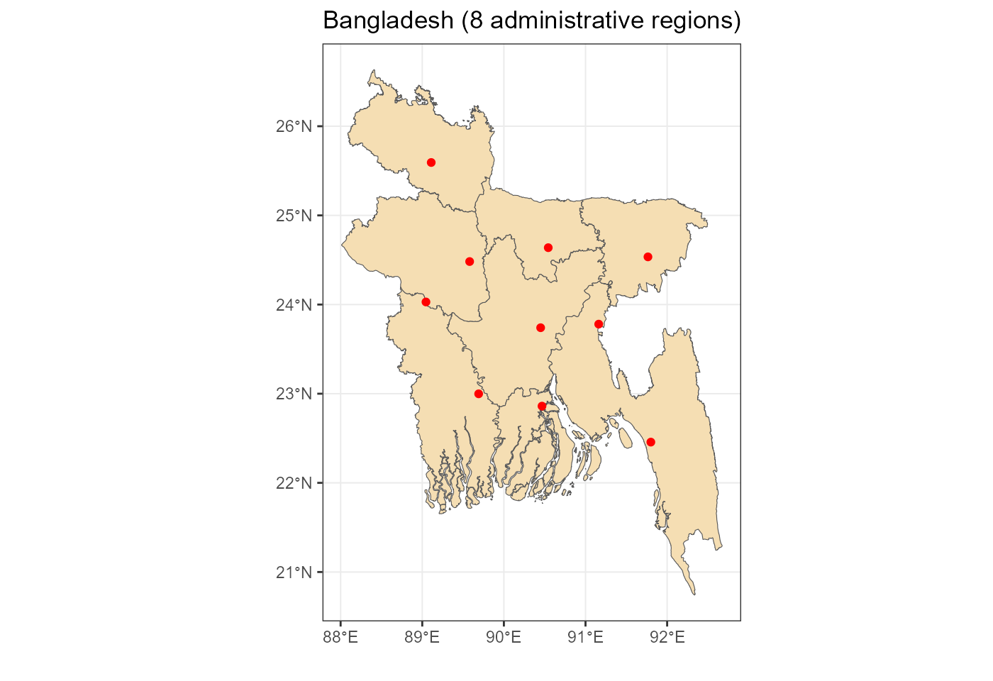

Voronoi clusters

This map with artificial regions have been created with “voronoi” algorithm around the simplified network nodes. The number of nodes is arbitrarily set to 10 (or 15 depending on country) to reduce dimension of the model for the first comparative runs. The network clustering is done by PyPSA-Earth framework and stored in the PyPSA folder (accessible to the project participants).
Key objects:
reg_nodes_sf - reg_nodes as sf object
gis$voronoi - added voronoi map to the gis list with maps
voronoi_map - ggplot map with voronoi clusters/regions around the given network nodes.

# voronoi map
reg_nodes_sf <- st_as_sf(reg_nodes, coords = c("lon", "lat"))
v <- reg_nodes_sf %>% 
  st_geometry() %>% 
  st_union() %>% 
  st_voronoi() 
st_crs(v) <- st_crs(gis$adm0$sf)
st_crs(reg_nodes_sf) <- st_crs(v)
if (!all(st_is_valid(v))) {
  v <- st_make_valid(v)
}
v <- rgeos::gIntersection(gis$adm0$sp, as_Spatial(st_cast(v)), 
                          byid = TRUE) %>% st_as_sf()
#> Warning: GEOS support is provided by the sf and terra packages among others
  
# v <- st_intersection(st_cast(v), st_union(gis$adm0$sf))
nn <- st_intersects(reg_nodes_sf, v) # mapping of nodes and polygons
v <- cbind(v[unlist(nn),], reg_nodes) # add nodes info
gis$voronoi <- list(sf = v, sp = as_Spatial(v)) # store for further use

voronoi_map <- ggplot(gis$voronoi$sf) +
  geom_sf(fill = "wheat") +
  geom_point(aes(lon, lat), col = "red") +
  labs(title = paste0(p$country, " (", nrow(reg_names), " clusters)"), 
       x = "", y = "") +
  # coord_sf(xlim = c(-80, -66), ylim = c(-55.5, -17.5)) +
  rev_theme_map()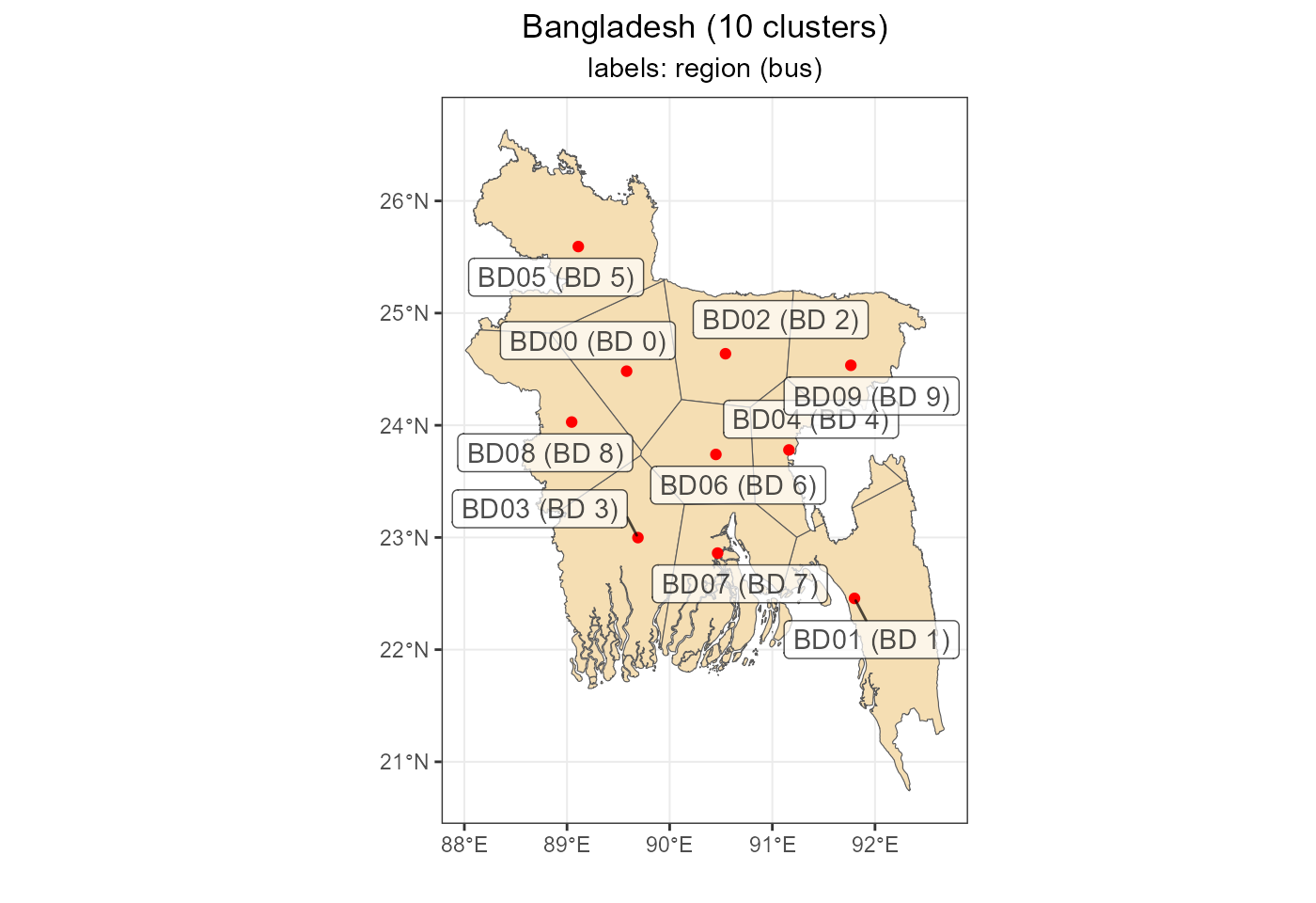

switch: load_zones.csv

Writing Switch input file with load_zones.

dir.create(file.path(p$switch$dir, "inputs"), showWarnings = F, recursive = T)
load_zones <- tibble(LOAD_ZONE = reg_names$load_zones)
stopifnot(!any(is.na((load_zones))))
write.csv(load_zones, 
          file = file.path(p$switch$dir, "inputs/load_zones.csv"), 
          row.names = FALSE, quote = FALSE)
head(load_zones, 3); cat("nrow = ", nrow(load_zones))
#> # A tibble: 3 × 1
#>   LOAD_ZONE
#>   <chr>    
#> 1 BD00     
#> 2 BD01     
#> 3 BD02
#> nrow =  10

timeslices / snapshots / timepoints

Time dimension in energyRt is set by years and hierarchical sub-annual dimensions (slices). In this project we use use three levels of slices: annual (“ANNUAL”), year-day (“YDAY”, from 1 to 365), and hour (“HOUR”, 0 to 23). The names and elements of all levels are already saved in revaluation::rev_data$tsl$d365_h24. The mapping with PyPSA’s “snapshots” are stored in revaluation::rev_data$timedim.

timedim <- rev_data$timedim %>% mutate(timepoints = slice)

switch: periods.csv

This table represent time-horizon in Switch.
The current model has only one (base) year for comparative reasons.

if (p$switch$import_pypsa) {
  ## switch: periods.csv ####
  periods <- tibble(
    INVESTMENT_PERIOD = p$base_year,
    period_start = p$base_year,
    period_end = p$base_year
  )
  stopifnot(!any(is.na(periods)))
  write.csv(periods, file = file.path(p$switch$dir, "inputs/periods.csv"), 
            row.names = FALSE, quote = FALSE)
}
periods
#> # A tibble: 1 × 3
#>   INVESTMENT_PERIOD period_start period_end
#>               <int>        <int>      <int>
#> 1              2018         2018       2018

switch: timeseries.csv

…

timeseries <- tibble(
  TIMESERIES = paste0(p$base_year, "_all"),
  ts_period = p$base_year,
  ts_duration_of_tp = 1L,
  ts_num_tps = 24L * 365L,
  ts_scale_to_period = 1L
)
stopifnot(!any(is.na((timeseries))))
write.csv(timeseries, file = file.path(p$switch$dir, "inputs/timeseries.csv"), 
          row.names = FALSE, quote = FALSE)
timeseries
#> # A tibble: 1 × 5
#>   TIMESERIES ts_period ts_duration_of_tp ts_num_tps ts_scale_to_period
#>   <chr>          <int>             <int>      <int>              <int>
#> 1 2018_all        2018                 1       8760                  1

switch: timepoints.csv

timepoints_map <- tibble(
  year = p$base_year, # assuming one year (temporary solution)
  slice = timedim$timepoints,
  timepoint_id = 
    paste(p$base_year,
      rep(
        timedim$timepoints,
        length(timeseries$TIMESERIES)
      ), sep = "_"
  ),
  timeseries = rep(
    timeseries$TIMESERIES, 
    each = length(timedim$timepoints)
  ),
  timestamp = "."
) %>%
  left_join(timedim, by = "slice")
timepoints <- timepoints_map %>% select(timepoint_id, timeseries, timestamp)
stopifnot(!any(is.na((timepoints))))
write.csv(timepoints, file = file.path(p$switch$dir, "inputs/timepoints.csv"),
          row.names = FALSE, quote = FALSE)
head(timepoints)
#> # A tibble: 6 × 3
#>   timepoint_id  timeseries timestamp
#>   <chr>         <chr>      <chr>    
#> 1 2018_d001_h00 2018_all   .        
#> 2 2018_d001_h01 2018_all   .        
#> 3 2018_d001_h02 2018_all   .        
#> 4 2018_d001_h03 2018_all   .        
#> 5 2018_d001_h04 2018_all   .        
#> 6 2018_d001_h05 2018_all   .

Commodities / carriers / energy sources

Commodities (energyRt) / carriers (PyPSA) / energy sources* (Switch)
* Switch recognizes fuels and non-fuel energy sources.

Key objects (created in the chunk below):
comm - a table with names of carriers, commodities

# create names of commodities
carriers <- nc$carriers %>%
  mutate(
    comm = carriers2comm(toupper(carriers_i)),
    drop = duplicated(comm) | is.na(comm)
  )

# drop duplicates, ...
comm <- filter(carriers, !drop) %>%
  # assign storage-commodity, slice-level, and supplied (market) commodity
  mutate(
    stg = grepl("HYD|PHS|H2|HGN|BTR", comm), # storage-commodity
    slice = if_else(stg, "HOUR", "ANNUAL"), # slice-level
    sup = grepl("ANNUAL", slice), # supplied commodity
    switch_nonfuel = carriers_co2_emissions == 0
  )

energyRt: commodities

# create commodities objects
ELC <- newCommodity("ELC", slice = "HOUR")
CO2 <- newCommodity("CO2", slice = "ANNUAL")
repo_comm <- newRepository("commodities", ELC, CO2)
if (nrow(comm) > 0) {
  for (i in 1:nrow(comm)) {
    com <- newCommodity(
      name = comm$comm[i],
      # description = comm$carriers_nice_name[i],
      slice = comm$slice[i],
      misc = list(color = comm$carriers_color[i])
    )
    if (comm$carriers_co2_emissions[i] != 0) {
      com <- update(com, 
                    emis = list(comm = "CO2", 
                                emis = comm$carriers_co2_emissions[i]))
    }
    repo_comm <- add(repo_comm, com)
    rm(com)
  }
} 
repo_comm@data %>% names()
#>  [1] "ELC" "CO2" "NUC" "GAS" "WIN" "BIO" "GEO" "SOL" "OIL" "COA" "LIG" "HYD"
#> [13] "PHS" "ROR" "H2"  "BTR"

switch: fuels.csv

Fuels in Switch model are energy sources with associated costs (by year and region, see “fuel_costs” module) and CO2 intensity. They cannot (!!!or can?) be considered as variable an energy source (example: coal, gas, biofuel).

fuels <- comm %>%
  filter(!switch_nonfuel | grepl("H2|BIO|NUC", comm)) %>%
  mutate(
    fuel = comm,
    co2_intensity = carriers_co2_emissions,
    upstream_co2_intensity = 0.
  ) %>%
  select(fuel, co2_intensity, upstream_co2_intensity)
stopifnot(!any(is.na((fuels))))
write.csv(fuels, file = file.path(p$switch$dir, "inputs/fuels.csv"),
          row.names = FALSE, quote = FALSE)
fuels
#>    fuel co2_intensity upstream_co2_intensity
#> 1:  NUC         0.000                      0
#> 2:  GAS         0.187                      0
#> 3:  BIO         0.000                      0
#> 4:  GEO         0.026                      0
#> 5:  OIL         0.248                      0
#> 6:  COA         0.354                      0
#> 7:  LIG         0.334                      0
#> 8:   H2         0.000                      0

switch: non_fuel_energy_sources.csv

This type indicates that the energy source can be variable (if declared in “gen_info” module and “variable_capacity_factors”); they don’t have associated costs, energy markets. Typical example: wind energy, solar energy, electricity.
Energy sources with (no costs in the model) and without variable capacity factors can be declared either as fuels or non-fuels. All declarations should be done only once.

## switch: non_fuel_energy_sources.csv ####
non_fuel_energy_sources <- comm %>%
  filter(!(comm %in% fuels$fuel)) %>%
  rename(energy_source = comm) %>%
  select(energy_source) %>%
  bind_rows(
    tibble(
      energy_source = c("Electricity")
    )) # ??? can it be ELC?

stopifnot(!any(is.na((non_fuel_energy_sources))))
write.csv(non_fuel_energy_sources, 
          file = file.path(p$switch$dir, "inputs/non_fuel_energy_sources.csv"),
          row.names = FALSE, quote = FALSE)
non_fuel_energy_sources
#>    energy_source
#> 1:           WIN
#> 2:           SOL
#> 3:           HYD
#> 4:           PHS
#> 5:           ROR
#> 6:           BTR
#> 7:   Electricity

Supply / markets

Supply (energyRt) / markets (Switch)

supp <- comm %>% filter(sup)

energyRt: supply

repo_sup <- newRepository("supply")
for (i in 1:nrow(supp)) {
  sup <- newSupply(
    name = paste0("SUP_", supp$comm[i]),
    commodity = supp$comm[i]
    # description = supp$carriers_nice_name[i],
  )
  repo_sup <- add(repo_sup, sup)
  rm(sup)
}
repo_sup@data %>% names()
#>  [1] "SUP_NUC" "SUP_GAS" "SUP_WIN" "SUP_BIO" "SUP_GEO" "SUP_SOL" "SUP_OIL"
#>  [8] "SUP_COA" "SUP_LIG" "SUP_ROR"

switch: fuel_cost.csv

# if (p$switch$import_pypsa) {
## switch: fuel_cost.csv ####
fuel_cost <- expand_grid(
  load_zone = reg_names$region, 
  fuel = fuels$fuel, # ??? can non-fuels be here?
  period = periods$INVESTMENT_PERIOD,
) %>%
mutate(
  fuel_cost = 0. # ??? No data in nc.file. Included in marginal costs?
)
stopifnot(!any(is.na(fuel_cost)))
write.csv(fuel_cost, 
          file = file.path(p$switch$dir, "inputs/fuel_cost.csv"),
          row.names = FALSE, quote = FALSE)
cat("file: inputs/fuel_cost.csv")
#> file: inputs/fuel_cost.csv
fuel_cost
#> # A tibble: 80 × 4
#>    load_zone fuel  period fuel_cost
#>    <chr>     <chr>  <int>     <dbl>
#>  1 BD00      NUC     2018         0
#>  2 BD00      GAS     2018         0
#>  3 BD00      BIO     2018         0
#>  4 BD00      GEO     2018         0
#>  5 BD00      OIL     2018         0
#>  6 BD00      COA     2018         0
#>  7 BD00      LIG     2018         0
#>  8 BD00      H2      2018         0
#>  9 BD01      NUC     2018         0
#> 10 BD01      GAS     2018         0
#> # … with 70 more rows

Demand / load profiles

Demand (energyRt) / loads (PyPSA & Switch) profiles

dem <- nc$loads %>%
  left_join(reg_names, by = c(loads_t_p_set_i = "bus")) %>%
  left_join(timedim, by = "snapshots") %>%
  mutate(
    yday = as.integer(str_extract(slice, "[0-9]++")),
    hour = as.integer(str_extract(slice, "[0-2][0-9]$")))

loads_byday <- dem %>%
  group_by(hour, region) %>%
  summarise(
    load_min = min(loads_t_p_set),
    load_max = max(loads_t_p_set),
    load_mean = mean(loads_t_p_set),
    .groups = "drop"
  )

fig_loads_hour <- ggplot(dem) +
  geom_line(aes(x = hour, y = loads_t_p_set/1e3, color = yday, group = yday),
            alpha = .5) +
  # geom_ribbon(aes(hour, ymin = load_min, ymax = load_max)) +
  scale_color_viridis_c(option = "H", name = "yday") +
  facet_wrap(~ region, ncol = 1, scales = "free_y", strip.position = "right") + 
  labs(x = "hour", y = "GWh", title = "Hourly load profile by day of the year") +
  rev_theme_map()

fig_loads_yday <- ggplot(dem) +
  geom_line(aes(x = yday, y = loads_t_p_set/1e3, color = hour, group = hour),
            alpha = .5) +
  # geom_ribbon(aes(hour, ymin = load_min, ymax = load_max)) +
  scale_color_viridis_c(option = "D", name = "hour", limits = c(0, 23)) +
  facet_wrap(~ region, ncol = 1, scales = "free_y", strip.position = "right") + 
  labs(x = "day of year (yday)", y = "GWh", 
       title = "Load profile by day of year and hour") +
  rev_theme_map()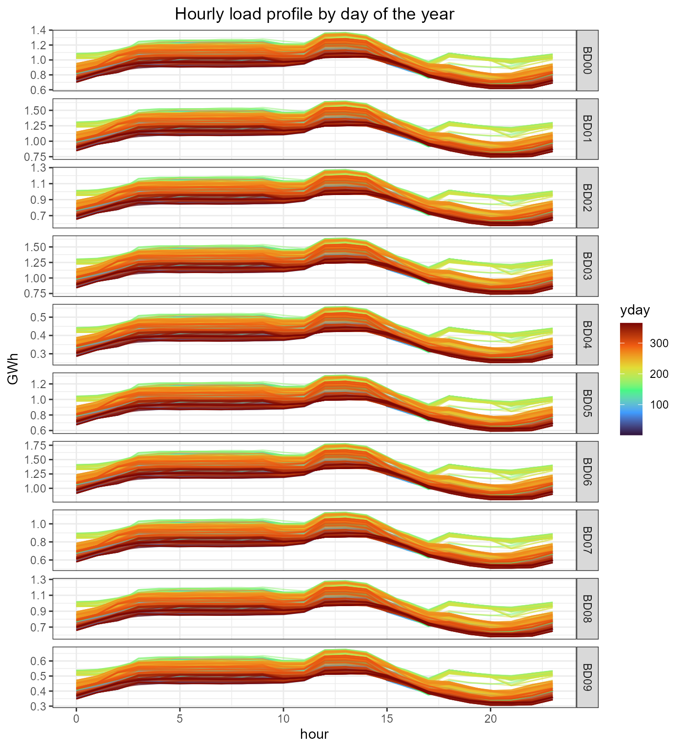

load_by_reg <- dem %>%
  group_by(region) %>%
  summarise(
    GWh = sum(loads_t_p_set, na.rm = T)/1e3,
    .groups = "drop"
  )

load_by_reg_sf <- gis$voronoi$sf %>%
  left_join(load_by_reg, by = "region")
  
fig_load_by_reg_sf <- ggplot(load_by_reg_sf) +
  geom_sf(aes(fill = GWh)) +
  scale_fill_viridis_c(option = "B") +
  labs(title = "Annual load by region/cluster") +
  rev_theme_map()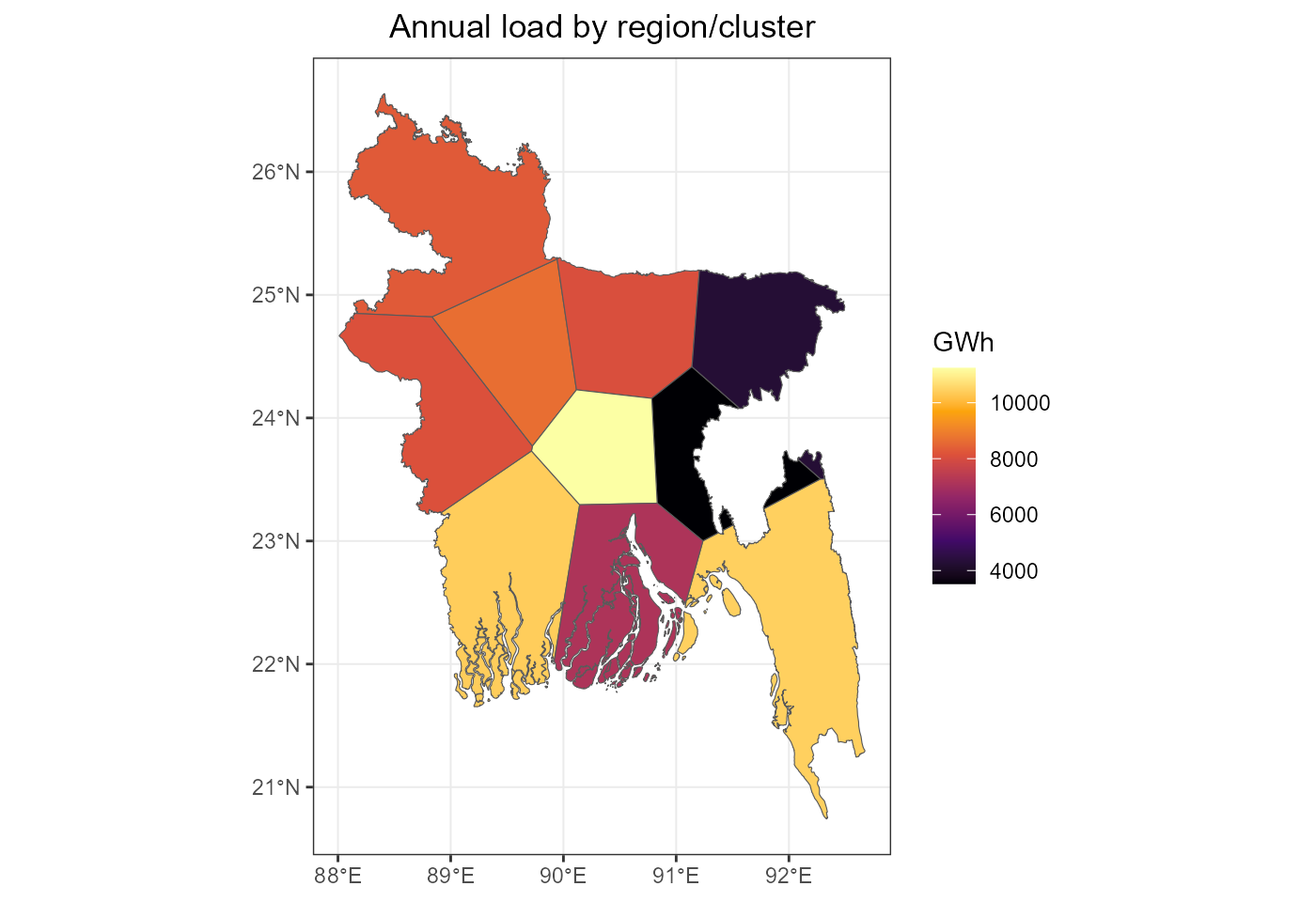

energyRt: demand

DEMELC <- newDemand(
  name = "DEMELC",
  description = "loads_t_p_set",
  commodity = "ELC",
  unit = "MWh",
  dem = list(
    region = dem$region,
    slice = dem$timepoints,
    dem = dem$loads_t_p_set
  )
)

switch: loads.csv

loads <- dem %>%
  left_join(
    select(timepoints_map, slice, timepoint_id),
    by = c(timepoints = "slice")) %>%
  mutate(
    LOAD_ZONE = region,
    TIMEPOINT = timepoint_id,
    zone_demand_mw = loads_t_p_set
  ) %>%
  select(LOAD_ZONE, TIMEPOINT, zone_demand_mw)
stopifnot(!any(is.na((loads))))
write.csv(loads, file = file.path(p$switch$dir, "inputs/loads.csv"), 
          row.names = FALSE, quote = FALSE)  
loads
#>        LOAD_ZONE     TIMEPOINT zone_demand_mw
#>     1:      BD00 2018_d001_h00       762.7098
#>     2:      BD01 2018_d001_h00       920.0083
#>     3:      BD02 2018_d001_h00       711.6408
#>     4:      BD03 2018_d001_h00       915.5576
#>     5:      BD04 2018_d001_h00       310.9402
#>    ---                                       
#> 87596:      BD05 2018_d365_h23       699.5984
#> 87597:      BD06 2018_d365_h23       947.4907
#> 87598:      BD07 2018_d365_h23       601.5130
#> 87599:      BD08 2018_d365_h23       684.0367
#> 87600:      BD09 2018_d365_h23       361.3412

Power network

network <- nc$lines %>% 
  left_join(reg_nodes, by = c("lines_bus0" = "bus")) %>%
  left_join(reg_nodes, by = c("lines_bus1" = "bus")) %>%
  mutate(
    losses = round(0.05 * lines_length / 1000, 3),
    trd_name = paste("TRL", region.x, region.y, sep = "_")
    ) # assuming 5% losses per 1000 km

net_map <- voronoi_map +
  geom_segment(aes(x = lon.x, y = lat.x, xend = lon.y, yend = lat.y), 
               data = network, color = "dodgerblue", linewidth = 2) +
  geom_point(aes(lon, lat), data = reg_nodes, col = "red") +
  geom_label_repel(aes(lon, lat, label = bus), data = reg_nodes, alpha = 0.7)

energyRt: trade

repo_network <- newRepository("network")
if (nrow(network) > 0) {
  for (i in 1:nrow(network)) {
    trd <- newTrade(
      name = network$trd_name[i],
      description = network$lines_type[i],
      commodity = "ELC",
      routes = data.frame(
        src = c(network$region.x[i], network$region.y[i]),
        dst = c(network$region.y[i], network$region.x[i])
      ),
      trade = data.frame(
        src = c(network$region.x[i], network$region.y[i]),
        dst = c(network$region.y[i], network$region.x[i]),
        teff = rep(1 - network$losses[i], 2)
      ),
      capacityVariable = T,
      invcost = data.frame(
        # costs can be assigned to one of the connected region or both
        # here we split the costs, 50% for each region
        region = c(network$region.x[i], network$region.y[i]),
        invcost = rep(network$lines_capital_cost[i] / 2, 2)
      ),
      stock = data.frame(
        # year = 
        stock = network$lines_s_nom[i]
      ),
      cap2act = 24*365
    )
    repo_network <- add(repo_network, trd)
    rm(trd)
  }
}
names(repo_network@data)
#>  [1] "TRL_BD00_BD02" "TRL_BD00_BD04" "TRL_BD00_BD05" "TRL_BD00_BD06"
#>  [5] "TRL_BD00_BD08" "TRL_BD01_BD04" "TRL_BD01_BD07" "TRL_BD02_BD04"
#>  [9] "TRL_BD03_BD07" "TRL_BD03_BD08" "TRL_BD04_BD06" "TRL_BD04_BD09"
#> [13] "TRL_BD06_BD07" "TRL_BD06_BD08" "TRL_BD06_BD09"

switch: transmission_lines.csv

Switch model considers transmission lines bi-directional. Key parameters:

transmission_lines <- tibble(
  TRANSMISSION_LINE = network$trd_name,
  trans_lz1 = network$region.x,
  trans_lz2 = network$region.y,
  trans_length_km = network$lines_length,
  trans_efficiency = 1 - network$losses,
  existing_trans_cap = network$lines_s_nom,
  trans_new_build_allowed = network$lines_s_nom_extendable
)
transmission_lines
#> # A tibble: 15 × 7
#>    TRANSMISSION_LINE trans_lz1 trans_lz2 trans_length_km trans…¹ exist…² trans…³
#>    <chr>             <chr>     <chr>               <dbl>   <dbl>   <dbl>   <int>
#>  1 TRL_BD00_BD02     BD00      BD02                124.    0.994    983.       1
#>  2 TRL_BD00_BD04     BD00      BD04                223.    0.989    983.       1
#>  3 TRL_BD00_BD05     BD00      BD05                165.    0.992   1966.       1
#>  4 TRL_BD00_BD06     BD00      BD06                151.    0.992    983.       1
#>  5 TRL_BD00_BD08     BD00      BD08                 92.6   0.995   2949.       1
#>  6 TRL_BD01_BD04     BD01      BD04                201.    0.99    1966.       1
#>  7 TRL_BD01_BD07     BD01      BD07                180.    0.991    983.       1
#>  8 TRL_BD02_BD04     BD02      BD04                143.    0.993    983.       1
#>  9 TRL_BD03_BD07     BD03      BD07                101.    0.995   2458.       1
#> 10 TRL_BD03_BD08     BD03      BD08                165.    0.992   2949.       1
#> 11 TRL_BD04_BD06     BD04      BD06                 90.7   0.995   9295.       1
#> 12 TRL_BD04_BD09     BD04      BD09                130.    0.994   1966.       1
#> 13 TRL_BD06_BD07     BD06      BD07                122.    0.994    983.       1
#> 14 TRL_BD06_BD08     BD06      BD08                183.    0.991    983.       1
#> 15 TRL_BD06_BD09     BD06      BD09                200.    0.99    3396.       1
#> # … with abbreviated variable names ¹​trans_efficiency, ²​existing_trans_cap,
#> #   ³​trans_new_build_allowed
stopifnot(!any(is.na((transmission_lines))))  
write.csv(transmission_lines, 
          file = file.path(p$switch$dir, "inputs/transmission_lines.csv"), 
          row.names = FALSE, quote = FALSE)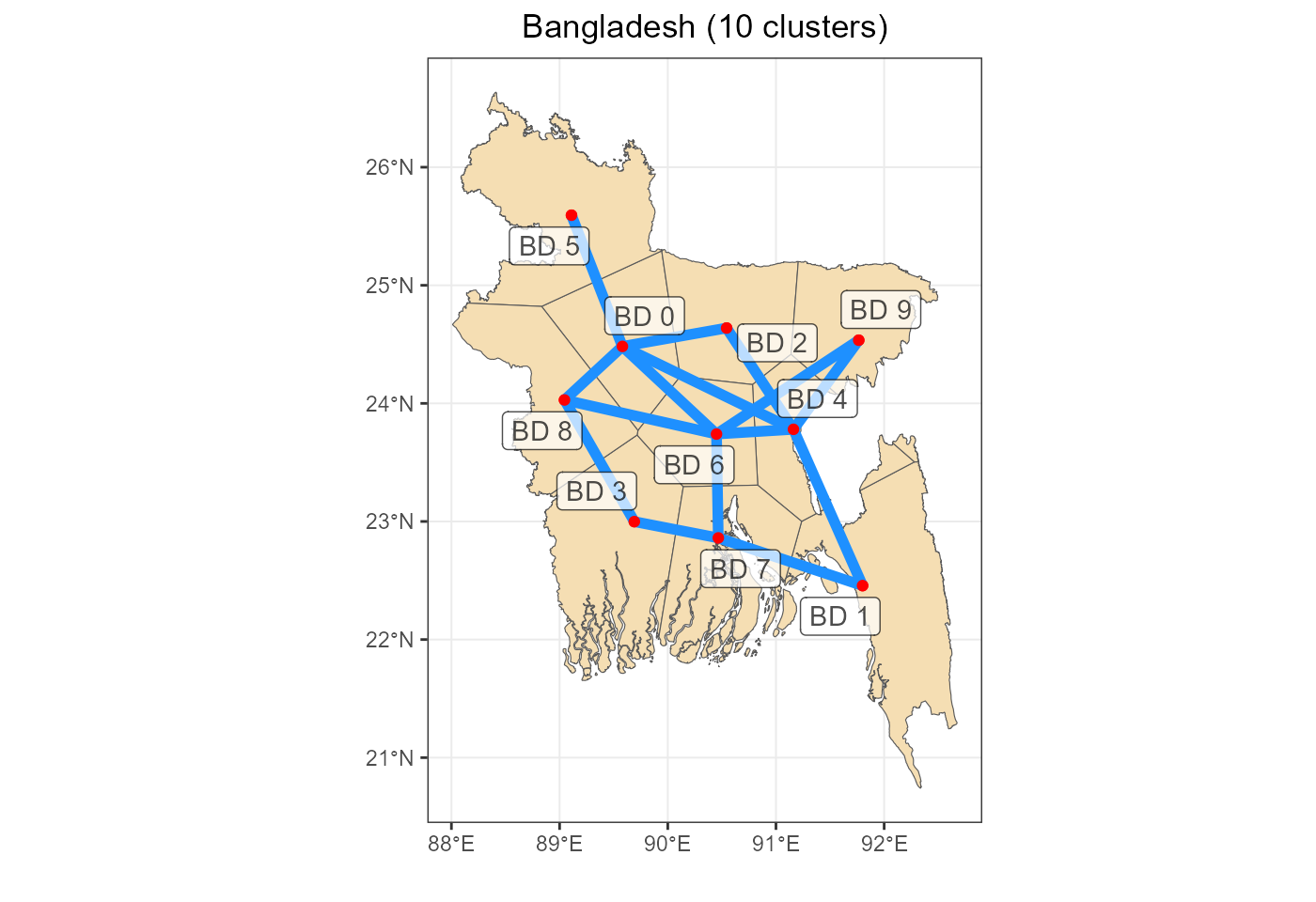  

Solar capacity factors

Weather factors (energyRt) / renewable profiles (PyPSA) / variable_capacity_factors (Switch).

solar <- nc$generators_cf %>%
  filter(grepl("[0-9] solar$", generators_t_p_max_pu_i)) %>%
  mutate( # !!! ToDo: write functions !!!
    bus = str_extract(generators_t_p_max_pu_i, "[A-Z]+.[0-9]+"),
    tech_pypsa = str_trim(str_replace(generators_t_p_max_pu_i, bus, "")),
    tech = "ESOL", # assuming one technology per region
    weather = "WSOL"
    ) %>%
  left_join(reg_names, by = "bus") %>%
  left_join(timedim, by = "snapshots")

solar_cf_sf <- solar %>%
  group_by(region) %>%
  summarise(
    cf = mean(generators_t_p_max_pu, na.rm = T), 
    .groups = "drop"
  )
solar_cf_sf <- gis$voronoi$sf %>%
  full_join(
    solar_cf_sf,
    by = "region")

fig_solar_cf_sf <- ggplot(solar_cf_sf) +
  geom_sf(aes(fill = cf)) +
  scale_fill_viridis_c(name = "CF", option = "C") +
  labs(title = "Solar annual average capacity factor") +
  rev_theme_map()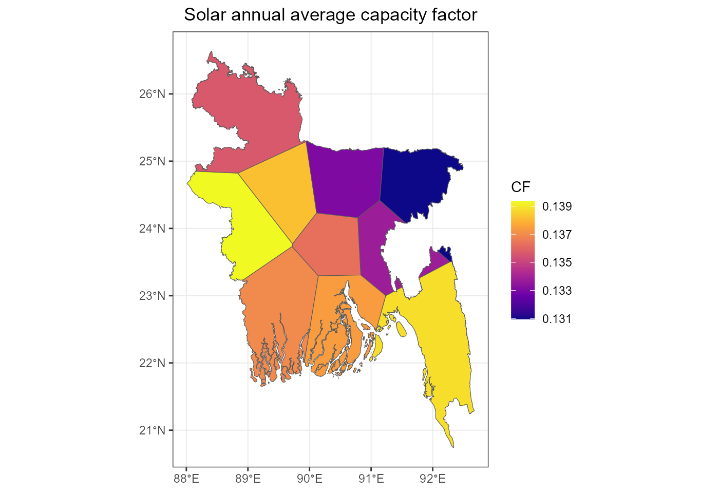

energyRt: weather factors (solar)

repo_solar_cf <- newRepository("repo_solar_cf")
if (nrow(solar) > 0) {
  for (w in unique(solar$weather)) {
    x <- filter(solar, weather %in% w)
    WSOL <- newWeather(
      name = w,
      description = "Solar generation profile",
      slice = "HOUR",
      weather = data.frame(
        region = x$region,
        slice = x$timepoints,
        wval = x$generators_t_p_max_pu
      )
    )
    repo_solar_cf <- add(repo_solar_cf, WSOL); rm(WSOL)
  }
}
repo_solar_cf@data %>% names()
#> [1] "WSOL"

switch: variable_capacity_factors (solar)

variable_capacity_factors_ESOL <- solar %>%
  left_join(timepoints_map, by = c("timepoints" = "slice")) %>%
  rename(
    timepoint = timepoint_id,
    gen_max_capacity_factor = generators_t_p_max_pu
  ) %>%
  mutate(
    GENERATION_PROJECT = paste0(region, "_ESOL")
  ) %>%
  select(GENERATION_PROJECT, timepoint, gen_max_capacity_factor)
variable_capacity_factors_ESOL
#>        GENERATION_PROJECT     timepoint gen_max_capacity_factor
#>     1:          BD00_ESOL 2018_d001_h00                       0
#>     2:          BD01_ESOL 2018_d001_h00                       0
#>     3:          BD02_ESOL 2018_d001_h00                       0
#>     4:          BD03_ESOL 2018_d001_h00                       0
#>     5:          BD04_ESOL 2018_d001_h00                       0
#>    ---                                                         
#> 87596:          BD05_ESOL 2018_d365_h23                       0
#> 87597:          BD06_ESOL 2018_d365_h23                       0
#> 87598:          BD07_ESOL 2018_d365_h23                       0
#> 87599:          BD08_ESOL 2018_d365_h23                       0
#> 87600:          BD09_ESOL 2018_d365_h23                       0

Onshore wind capacity factors

onwind <- nc$generators_cf %>%
  filter(grepl("[0-9] onwind$", generators_t_p_max_pu_i)) %>%
  mutate( # !!! ToDo: write functions !!!
    bus = str_extract(generators_t_p_max_pu_i, "[A-Z]+.[0-9]+"),
    tech_pypsa = str_trim(str_replace(generators_t_p_max_pu_i, bus, "")),
    tech = "EWIN", # assuming one technology per region
    weather = "WWIN") %>%
  left_join(reg_names, by = "bus") %>%
  left_join(timedim, by = "snapshots")

onwind_cf_sf <- onwind %>%
  group_by(region) %>%
  summarise(
    cf = mean(generators_t_p_max_pu, na.rm = T), 
    .groups = "drop"
  )
onwind_cf_sf <- gis$voronoi$sf %>%
  full_join(
    onwind_cf_sf,
    by = "region")

fig_onwind_cf_sf <- ggplot(onwind_cf_sf) +
  geom_sf(aes(fill = cf)) +
  scale_fill_viridis_c(name = "CF", option = "D") +
  labs(title = "Wind annual average capacity factor") +
  rev_theme_map()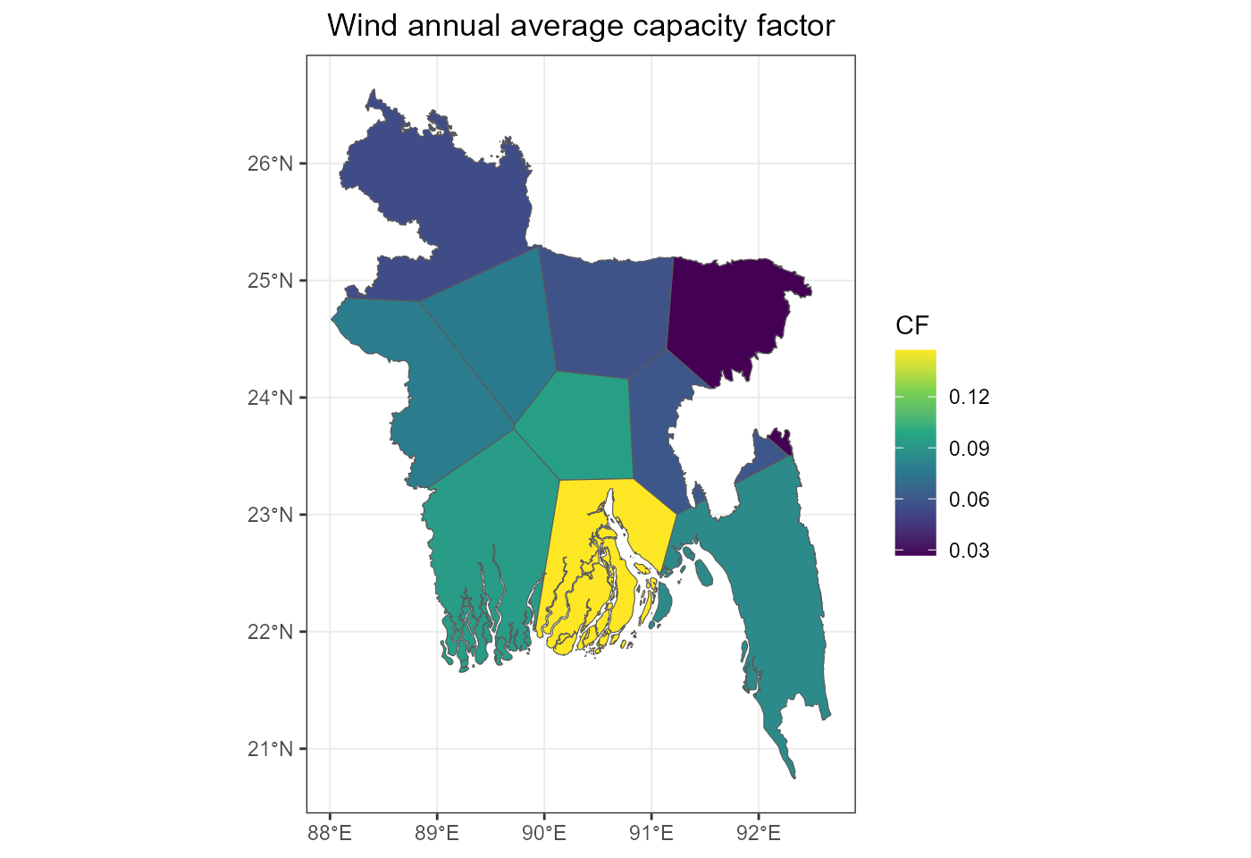

energyRt: weather factors (onshore wind)

repo_onwind_cf <- newRepository("repo_onwind_cf")
if (nrow(onwind) > 0) {
  for (w in unique(onwind$weather)) {
    x <- filter(onwind, weather %in% w)
    WWIN <- newWeather(
      name = w,
      description = "Onshore wind generation profile",
      slice = "HOUR",
      weather = data.frame(
        region = x$region,
        slice = x$timepoints,
        wval = x$generators_t_p_max_pu
      )
    )
    repo_onwind_cf <- add(repo_onwind_cf, WWIN); rm(WWIN)
  }
}
repo_onwind_cf@data %>% names()
#> [1] "WWIN"

switch: variable_capacity_factors (onshore wind)

variable_capacity_factors_EWIN <- onwind %>%
  left_join(timepoints_map, by = c("timepoints" = "slice")) %>%
  rename(
    timepoint = timepoint_id,
    gen_max_capacity_factor = generators_t_p_max_pu
  ) %>%
  mutate(
    GENERATION_PROJECT = paste0(region, "_EWIN")
  ) %>%
  select(GENERATION_PROJECT, timepoint, gen_max_capacity_factor)
variable_capacity_factors_EWIN
#>        GENERATION_PROJECT     timepoint gen_max_capacity_factor
#>     1:          BD00_EWIN 2018_d001_h00             0.007937158
#>     2:          BD01_EWIN 2018_d001_h00             0.067636342
#>     3:          BD02_EWIN 2018_d001_h00             0.002534725
#>     4:          BD03_EWIN 2018_d001_h00             0.000000000
#>     5:          BD04_EWIN 2018_d001_h00             0.004233536
#>    ---                                                         
#> 87596:          BD05_EWIN 2018_d365_h23             0.013626025
#> 87597:          BD06_EWIN 2018_d365_h23             0.076793543
#> 87598:          BD07_EWIN 2018_d365_h23             0.108927167
#> 87599:          BD08_EWIN 2018_d365_h23             0.067855158
#> 87600:          BD09_EWIN 2018_d365_h23             0.000000000

Hydro (ror) capacity factors

ror <- nc$generators_cf %>%
  filter(grepl("[0-9] ror$", generators_t_p_max_pu_i)) %>%
  mutate( # !!! ToDo: write functions !!!
    bus = str_extract(generators_t_p_max_pu_i, "[A-Z]+.[0-9]+"),
    tech_pypsa = str_trim(str_replace(generators_t_p_max_pu_i, bus, "")),
    tech = "EROR", # assuming one technology per region
    weather = "WROR") %>%
  left_join(reg_names, by = "bus") %>%
  left_join(timedim, by = "snapshots")

unique(ror$generators_t_p_max_pu_i)
#> character(0)
unique(ror$bus)
#> character(0)
ror_cf_sf <- ror %>%
  group_by(region) %>%
  summarise(
    cf = mean(generators_t_p_max_pu, na.rm = T), 
    .groups = "drop"
  )
ror_cf_sf <- gis$voronoi$sf %>%
  full_join(
    ror_cf_sf,
    by = "region")

fig_ror_cf_sf <- ggplot(ror_cf_sf) +
  geom_sf(aes(fill = cf)) +
  scale_fill_viridis_c(name = "CF", option = "D") +
  labs(title = "Hydro (ROR) annual average capacity factor") +
  rev_theme_map()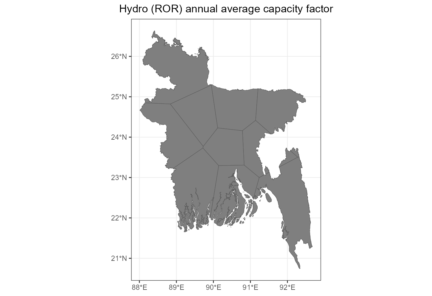

energyRt: weather factors (run of river)

repo_ror_cf <- newRepository("repo_ror_cf")
if (nrow(ror) > 0) {
  for (w in unique(ror$weather)) {
    x <- filter(ror, weather %in% w)
    WROR <- newWeather(
      name = w,
      description = "Run of river hydro generation profile",
      slice = "HOUR",
      weather = data.frame(
        region = x$region,
        slice = x$timepoints,
        wval = x$generators_t_p_max_pu
      )
    )
    repo_ror_cf <- add(repo_ror_cf, WROR); rm(WROR)
  }
}
repo_ror_cf@data %>% names()
#> NULL

switch: variable_capacity_factors (run of river)

variable_capacity_factors_EROR <- ror %>%
  left_join(timepoints_map, by = c("timepoints" = "slice")) %>%
  rename(
    timepoint = timepoint_id,
    gen_max_capacity_factor = generators_t_p_max_pu
  ) %>%
  mutate(
    GENERATION_PROJECT = paste0(region, "_EROR")
  ) %>%
  select(GENERATION_PROJECT, timepoint, gen_max_capacity_factor)
variable_capacity_factors_EROR
#> Empty data.table (0 rows and 3 cols): GENERATION_PROJECT,timepoint,gen_max_capacity_factor

switch: variable_capacity_factors.csv

Combine all capacity factors of variable technologies and write the csv-file.

variable_capacity_factors <- variable_capacity_factors_ESOL %>%
  rbind(variable_capacity_factors_EWIN) %>%
  rbind(variable_capacity_factors_EROR)

# checks
variable_capacity_factors %>% summary()
#>  GENERATION_PROJECT  timepoint         gen_max_capacity_factor
#>  Length:175200      Length:175200      Min.   :0.00000        
#>  Class :character   Class :character   1st Qu.:0.00000        
#>  Mode  :character   Mode  :character   Median :0.02601        
#>                                        Mean   :0.10662        
#>                                        3rd Qu.:0.14775        
#>                                        Max.   :0.99971
variable_capacity_factors$GENERATION_PROJECT %>% unique()
#>  [1] "BD00_ESOL" "BD01_ESOL" "BD02_ESOL" "BD03_ESOL" "BD04_ESOL" "BD05_ESOL"
#>  [7] "BD06_ESOL" "BD07_ESOL" "BD08_ESOL" "BD09_ESOL" "BD00_EWIN" "BD01_EWIN"
#> [13] "BD02_EWIN" "BD03_EWIN" "BD04_EWIN" "BD05_EWIN" "BD06_EWIN" "BD07_EWIN"
#> [19] "BD08_EWIN" "BD09_EWIN"
str_replace(variable_capacity_factors$GENERATION_PROJECT, 
            "^[A-Z]+[0-9]+_", "") %>% unique()
#> [1] "ESOL" "EWIN"
# stopifnot(!any(is.na((variable_capacity_factors))  
write.csv(variable_capacity_factors,
          file = file.path(p$switch$dir, "inputs/variable_capacity_factors.csv"),
          row.names = FALSE, quote = FALSE)
variable_capacity_factors
#>         GENERATION_PROJECT     timepoint gen_max_capacity_factor
#>      1:          BD00_ESOL 2018_d001_h00              0.00000000
#>      2:          BD01_ESOL 2018_d001_h00              0.00000000
#>      3:          BD02_ESOL 2018_d001_h00              0.00000000
#>      4:          BD03_ESOL 2018_d001_h00              0.00000000
#>      5:          BD04_ESOL 2018_d001_h00              0.00000000
#>     ---                                                         
#> 175196:          BD05_EWIN 2018_d365_h23              0.01362603
#> 175197:          BD06_EWIN 2018_d365_h23              0.07679354
#> 175198:          BD07_EWIN 2018_d365_h23              0.10892717
#> 175199:          BD08_EWIN 2018_d365_h23              0.06785516
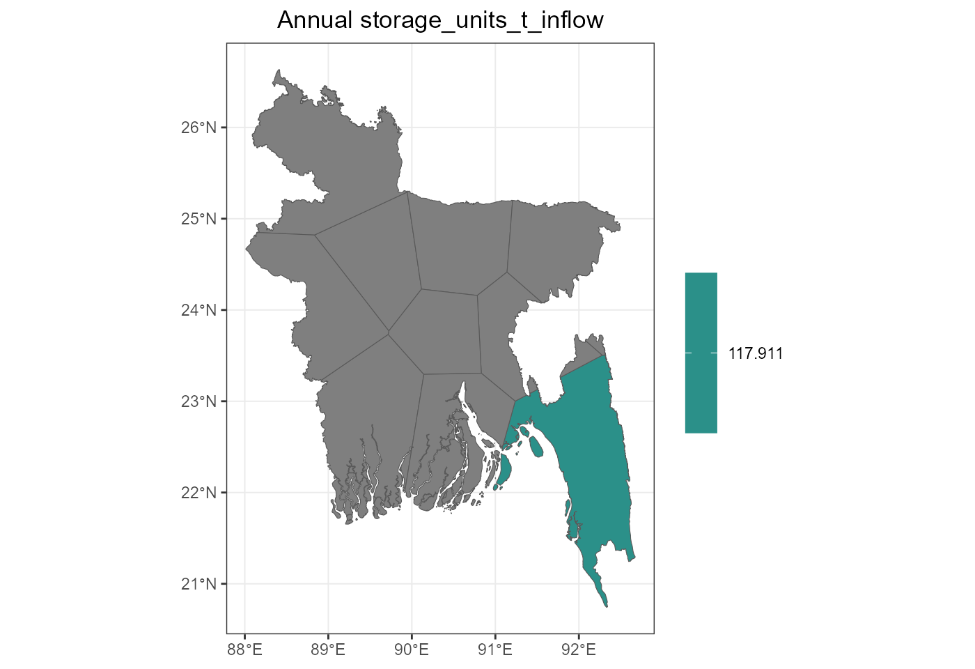
#> 175200:          BD09_EWIN 2018_d365_h23              0.00000000

Hydro inflow

Those time series can be used to control charging process in energyRt in storage or supply type of processes, or in generators in Switch or energyRt.

inflow <- nc$storage_inflow %>%
  mutate( # !!! ToDO: write functions !!!
    bus = str_extract(storage_units_t_inflow_i, "[A-Z]+.[0-9]+"),
    storage = str_trim(str_replace(storage_units_t_inflow_i, bus, "")),
    comm = str_sub(toupper(storage), 1, 3),
    stg = paste0("STG_", comm), # in the case it is used in storage class objects
    sup = paste0("SUP_", comm), # in the case it is used in supply class objects
    weather = paste0("W", comm)  # 
  ) %>%
  left_join(reg_names, by = "bus") %>%
  left_join(timedim, by = "snapshots")

if (nrow(inflow) > 0) {
  unique(inflow$bus)
  unique(inflow$stg)
  unique(inflow$weather)

  inflow_sf <- inflow %>%
    group_by(region) %>%
    summarise(
      storage_units_t_inflow = mean(storage_units_t_inflow, na.rm = T), 
      .groups = "drop"
    )
  inflow_sf <- gis$voronoi$sf %>%
    full_join(
      inflow_sf,
      by = "region")
  
  fig_inflow_sf <- ggplot(inflow_sf) +
    geom_sf(aes(fill = storage_units_t_inflow)) +
    scale_fill_viridis_c(name = "", option = "D") +
    labs(title = "Annual storage_units_t_inflow") +
    rev_theme_map()
}

energyRt: weather factors (hydro storage inflow)

repo_inflow <- newRepository("repo_inflow")
if (nrow(inflow) > 0) {
  for (w in unique(inflow$weather)) {
    x <- filter(inflow, weather %in% w)
    WHYD <- newWeather(
      name = w,
      description = "Hydro inflow profile",
      slice = "HOUR",
      weather = data.frame(
        region = x$region,
        slice = x$timepoints,
        wval = x$storage_units_t_inflow
      )
    )
    repo_inflow <- add(repo_inflow, WHYD); rm(WHYD)
  }
}
repo_inflow@data %>% names()
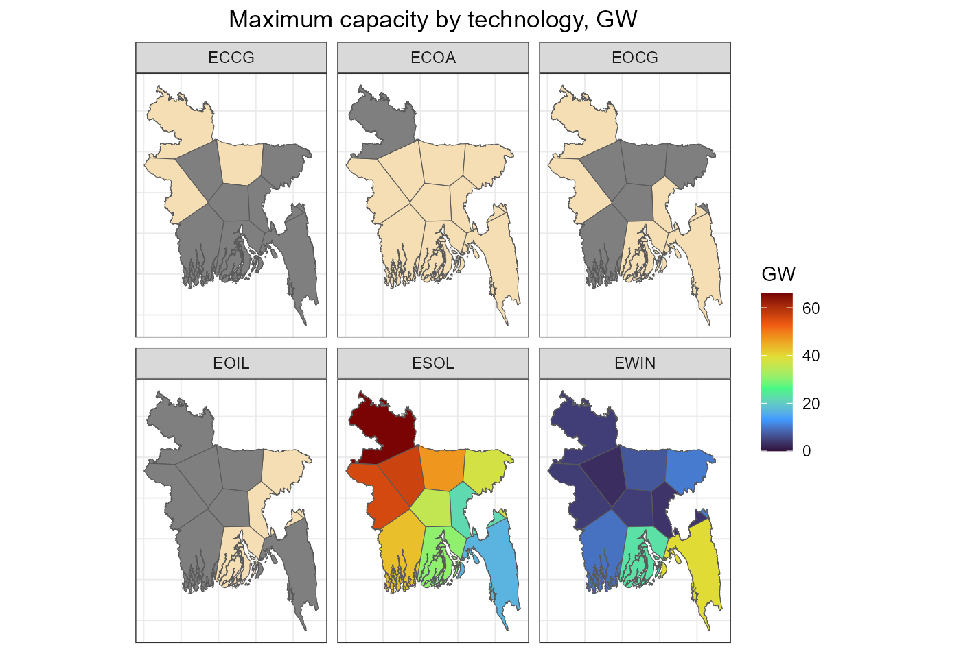
#> [1] "WHYD"

Generators

gen <- nc$generators %>%
  # filter(grepl("[0-9] onwind$", generators_t_p_max_pu_i)) %>%
  mutate(
    bus = str_extract(generators_i, "[A-Z]+.[0-9]+"),
    comm = carriers2comm(generators_i),
    gen = str_replace(generators_i, bus, ""),
    gen = str_trim(gen),
    tech_name = substr(paste0("E", toupper(gen)), 1, 4) # !!! ToDo: Write a function
  ) %>%
  left_join(reg_names, by = "bus")
gen$tech_name[grepl("EONW", gen$tech_name)] <- "EWIN" # !!! ToDo: Write a function
gen$tech_name %>% unique()
#> [1] "ECCG" "EOCG" "EOIL" "EWIN" "ESOL" "ECOA"

gen_sf <- gen %>%
  group_by(region, tech_name) %>%
  summarise(
    GW = sum(generators_p_nom, na.rm = T)/1e3, 
    GW_max = sum(generators_p_nom_max , na.rm = T)/1e3,
    .groups = "drop"
  )
gen_sf <- gis$voronoi$sf %>%
  full_join(
    gen_sf,
    by = "region")
#> Warning in sf_column %in% names(g): Each row in `x` is expected to match at most 1 row in `y`.
#> ℹ Row 1 of `x` matches multiple rows.
#> ℹ If multiple matches are expected, set `multiple = "all"` to silence this
#>   warning.

fig_gen_cap <- ggplot() +
  geom_sf(data = gis$voronoi$sf, fill = "wheat") +
  geom_sf(aes(fill = GW), data = gen_sf) +
  scale_fill_viridis_c(name = "GW", option = "H", limits = c(0, NA)) +
  labs(title = "Existing (installed) generators, GW") +
  facet_wrap(~tech_name) +
  rev_theme_map() +
  theme(axis.text.x = element_blank(), axis.ticks.x = element_blank(), 
        axis.text.y = element_blank(), axis.ticks.y = element_blank())

fig_gen_cap_max <- ggplot() +
  geom_sf(data = gis$voronoi$sf, fill = "wheat") +
  geom_sf(aes(fill = GW_max), data = gen_sf) +
  scale_fill_viridis_c(name = "GW", option = "H", limits = c(0, NA)) +
  labs(title = "Maximum capacity by technology, GW") +
  facet_wrap(~tech_name) +
  rev_theme_map() +
  theme(axis.text.x = element_blank(), axis.ticks.x = element_blank(), 
        axis.text.y = element_blank(), axis.ticks.y = element_blank())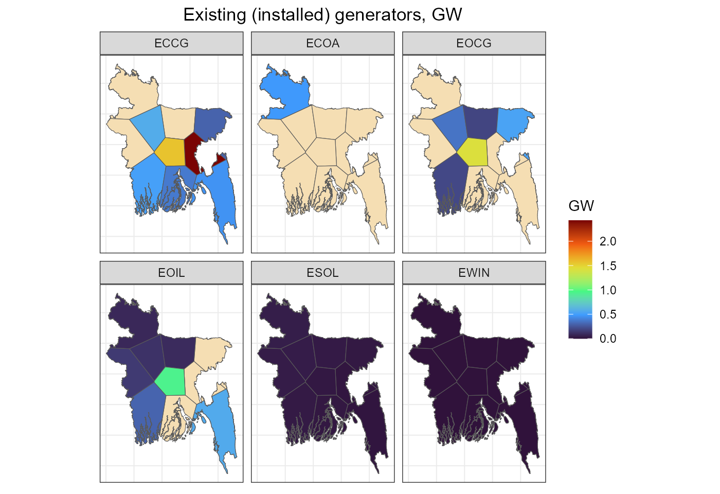

energyRt: technologies (generators)

repo_gen <- newRepository("generators")
for (tch in unique(gen$tech_name)) {
  x <- gen %>% filter(tech_name == tch)
  tech <- newTechnology(
    name = tch,
    description = x$generators_i[1],
    # description = paste(x$generators_i, collapse = ", "),
    input = list(comm = unique(x$comm)),
    output = list(comm = "ELC"),
    cap2act = 24*365,
    region = unique(x$region),
    ceff = list(
      region = x$region,
      comm = x$comm,
      cinp2use = x$generators_efficiency
    ),
    invcost = list(
      region = x$region,
      invcost = x$generators_capital_cost
    ),
    varom = list(
      region = x$region,
      varom = x$generators_marginal_cost
    ),
    stock = list(
      region = x$region,
      stock = x$generators_p_nom
    )
  )
  if (grepl("solar", tch, ignore.case = T)) {
    tech <- update(tech, weather = list(weather = "WSOL", waf.fx = 1))
  } else if (grepl("onwind", tch, ignore.case = T)) {
    tech <- update(tech, weather = list(weather = "WWIN", waf.fx = 1))
  } else if (grepl("ror", tch, ignore.case = T)) {
    tech <- update(tech, weather = list(weather = "WROR", waf.fx = 1))
  }
  # availability of the technology for investment
  extendable <- x$generators_p_nom_extendable
  if (any(extendable != 1)) {
    if (!any(extendable == 1 | extendable == 0)) {
      # error in the data
      print(x)
      stop("Unexpected value in 'generators_p_nom_extendable' {0 or 1}")
    }
   tech <- update(
     tech, 
     end = list(
       region = x$region,
       end = if_else(
         x$generators_p_nom_extendable == 1,
         p$base_year, # open for investment
         p$base_year - 1 # not available for investment
        )
      )
    )
  }
  repo_gen <- add(repo_gen, tech)
}
names(repo_gen@data)
#> [1] "ECCG" "EOCG" "EOIL" "EWIN" "ESOL" "ECOA"
try(draw(repo_gen@data[[1]]))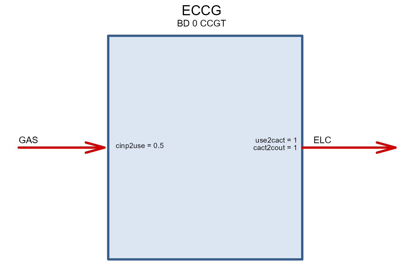

switch: gen_info (generators)

gen_info_tech <- gen %>%
  mutate(
    GENERATION_PROJECT = paste0(region, "_", tech_name),
    gen_tech = tech_name,
    gen_load_zone = region,
    gen_connect_cost_per_mw = 0.,
    gen_capacity_limit_mw = generators_p_nom_max, # ".",
    gen_full_load_heat_rate = as.character(
      round(
        convert("GWh/GWh", "MMBtu/MWh", 1 / generators_efficiency), 3)),
    gen_variable_om = generators_marginal_cost,
    gen_max_age = 1, # !!! ToDo: convert to overnight costs
    gen_is_variable = 
      as.integer(
        grepl("ECSP|ESPV|ESOL|EWIN|EWIF|EROR|EHYD", tech_name)), # !!! ToDo: Write function
    gen_full_load_heat_rate = 
      if_else(gen_is_variable == 1, ".", gen_full_load_heat_rate),
    gen_is_baseload = as.integer(!as.logical(gen_is_variable)),
    gen_is_cogen = 0L,
    gen_energy_source   = comm,
    gen_store_to_release_ratio = ".",
    gen_storage_efficiency = ".",
     # gen_unit_size    gen_ccs_capture_efficiency  gen_ccs_energy_load
  )

gen_info_tech$gen_full_load_heat_rate[
  gen_info_tech$gen_is_variable == 1] <- "." 

gen_info_tech$gen_capacity_limit_mw[
  is.infinite(gen_info_tech$gen_capacity_limit_mw)] <- "."

gen_info_csv <- gen_info_tech %>%
  select(GENERATION_PROJECT:gen_storage_efficiency)
gen_info_csv$gen_tech %>% unique()
#> [1] "ECCG" "EOCG" "EOIL" "EWIN" "ESOL" "ECOA"
stopifnot(!any(is.na((gen_info_csv))))

switch: gen_build_predetermined (generators)

if (nrow(gen_info_tech) > 0) {
  gen_build_predetermined_tech <- gen_info_tech %>%
    filter(generators_p_nom > 0 | generators_p_nom_extendable == 0) %>%
    mutate(
      build_year = p$base_year - 1,
      build_gen_predetermined = generators_p_nom
    ) %>%
    select(GENERATION_PROJECT, build_year, build_gen_predetermined)

  gen_build_predetermined <- gen_build_predetermined_tech
  # stopifnot(!any(is.na((gen_build_predetermined))))
} else {
  gen_build_predetermined <- NULL
}

switch: gen_build_costs (generators)

gen_build_costs <- gen_info_tech %>%
  mutate(
    build_year = NA,
    gen_overnight_cost = generators_capital_cost,
    gen_fixed_om = 0L,
    gen_storage_energy_overnight_cost = "."
  ) %>%
  select(GENERATION_PROJECT, build_year, gen_overnight_cost, gen_fixed_om,
         gen_storage_energy_overnight_cost)

# costs of existing stock
gen_build_costs_0 <- gen_build_costs %>%
  filter(GENERATION_PROJECT %in% gen_build_predetermined$GENERATION_PROJECT) %>%
  mutate(
    build_year = p$base_year - 1
  )

# investable 
gen_build_costs_1 <- gen_build_costs %>%
  filter(
    GENERATION_PROJECT %in% 
      gen_info_tech$GENERATION_PROJECT[
        gen_info_tech$generators_p_nom_extendable == 1]) %>%
  mutate(
    build_year = p$base_year
  )
# merge
gen_build_costs <- rbind(gen_build_costs_0, gen_build_costs_1)
rm(gen_build_costs_0, gen_build_costs_1)
gen_build_costs$GENERATION_PROJECT %>% unique()
#>  [1] "BD00_ECCG" "BD00_EOCG" "BD00_EOIL" "BD00_ESOL" "BD01_ECCG" "BD01_EOIL"
#>  [7] "BD01_EWIN" "BD01_ESOL" "BD02_EOCG" "BD02_EOIL" "BD02_ESOL" "BD03_ECCG"
#> [13] "BD03_EOCG" "BD03_EOIL" "BD03_ESOL" "BD04_ECCG" "BD04_ESOL" "BD05_ECOA"
#> [19] "BD05_EOIL" "BD05_ESOL" "BD06_ECCG" "BD06_EOCG" "BD06_EOIL" "BD06_ESOL"
#> [25] "BD07_ECCG" "BD07_EWIN" "BD07_ESOL" "BD08_EOIL" "BD08_ESOL" "BD09_ECCG"
#> [31] "BD09_EOCG" "BD09_ESOL" "BD00_EWIN" "BD02_EWIN" "BD03_EWIN" "BD04_EWIN"
#> [37] "BD05_EWIN" "BD06_EWIN" "BD08_EWIN" "BD09_EWIN"

stopifnot(!any(is.na((gen_build_costs))))
head(gen_build_costs)
#>    GENERATION_PROJECT build_year gen_overnight_cost gen_fixed_om
#> 1:          BD00_ECCG       2017           84469.12            0
#> 2:          BD00_EOCG       2017           47234.56            0
#> 3:          BD00_EOIL       2017           38234.56            0
#> 4:          BD00_ESOL       2017           55064.07            0
#> 5:          BD01_ECCG       2017           84469.12            0
#> 6:          BD01_EOIL       2017           38234.56            0
#>    gen_storage_energy_overnight_cost
#> 1:                                 .
#> 2:                                 .
#> 3:                                 .
#> 4:                                 .
#> 5:                                 .
#> 6:                                 .

Storage types

There are several types of storage in the current PyPSA-Earth models:

1. accumulators (of a carrier):

• data table: nc$stores
• carrier: “battery” or “H2” (electricity or hydrogen)
• no existing capacity (can be added later)
• capital costs: stores_capital_cost
• efficiency: 100% (losses are modeled via “links”: chargers and dischargers)

2. pumped hydro

• data table: nc$storage_units
• carrier: “PHS”
• storage_units_capital_cost
• storage_units_efficiency_dispatch
• storage_units_efficiency_store (!!!units? charging efficiency or storing?)

3. hydro power plant (PP) with a dam and exogenous inflow:

• data tables:
  • nc$storage_units_set - sets
  • nc$storage_units - parameters
  • nc$storage_inflow - exogenous inflow factors
• carrier: “hydro”
• storage_units_p_nom - existing electric capacity
• storage_units_max_hours - storage capacity parameter
• storage_units_efficiency_dispatch
  Note: the listed types of storage are model/scenario-specific, not generic.

Accumulators

Modeled as a generic storage, the model optimizes energy capacity (MWh). Efficiency is assumed 100%, losses are modeled via links (“chargers” and “dischargers” for electricity, “electrolysis” and “fuel cells” for hydrogen).

storage <- nc$stores %>%
  mutate(
    bus = str_extract(stores_bus, "[A-Z]+.[0-9]+"),
    comm = carriers2comm(stores_carrier),
    stores = str_replace(stores_i, bus, ""),
    stores = str_trim(stores),
    # stg_name = paste0("STG_", toupper(stores))
    # storage = str_trim(str_replace(storage_units_t_inflow_i, bus, "")),
    comm = str_sub(toupper(stores), 1, 3),
    stg = paste0("STG_", comm),
    comm = str_replace(comm, "^BAT$", "ELC"),
    stg = str_replace(stg, "_BAT", "_BTR")
  ) %>%
  left_join(reg_names, by = "bus")
# storage
cat("Found", length(unique(storage$stg)), 
    "stores (accumulators) for carriers:\n");unique(storage$stores_carrier)
#> Found 2 stores (accumulators) for carriers:
#> [1] "H2"      "battery"
cat("Storage technologies names to create in energyRt:\n");unique(storage$stg)
#> Storage technologies names to create in energyRt:
#> [1] "STG_H2"  "STG_BTR"

energyRt: storage (accumulators)

repo_stg <- newRepository("storages")
if (nrow(storage) > 0) {
  for (s in unique(storage$stg)) {
    x <- storage %>% filter(stg == s)
    stg <- newStorage(
      name = s,
      # description = paste(x$stores_i, collapse = ", "),
      commodity = list(comm = unique(x$comm)),
      # cap2act = 24*365,
      region = unique(x$region),
      invcost = list(
        region = x$region,
        invcost = x$stores_capital_cost
      )
    )
  # availability of the technology for investment
    extendable <- x$stores_e_nom_extendable
    if (any(extendable != 1)) {
      if (!any(extendable == 1 | extendable == 0)) { # check for errors
        # error in the data
        print(x)
        stop("Unexpected value in 'stores_e_nom_extendable' {0 or 1}")
      }
      stg <- update(
        stg, 
        end = list(
          region = x$region,
          end = if_else(
            x$stores_e_nom_extendable == 1,
            p$base_year, # open for investment
            p$base_year - 1 # not available for investment
          )
        )
      )
    }    
    repo_stg <- add(repo_stg, stg); rm(stg)
  }
}
repo_stg@data %>% names()
#> [1] "STG_H2"  "STG_BTR"

Note: Accumulators in Switch are modeled together with “links” (chargers and dischargers) below.

Pumped hydro (PHS)

This type of storage in PyPSA-Earth has hydro as an storage_units_carrier. Though if availability of hydro is not linked with the ability to accumulate (!check!), then the modeling of the carrier can be avoided. The storage itself can be represented as an electricity storage with overall storage capacity equal to storage_units_p_nom * storage_units_max_hours in MWh where storage_units_p_nom is discharge capacity in MW. This approach is straightforward to reproduce in both Switch and energyRt. A version with hydro carrier can also be modeled, but may require advanced hydro module (will be considered later).

unique(nc$storage_units$storage_units_carrier)
#> [1] "hydro"
phs <- nc$storage_units %>%
  filter(grepl("PHS", storage_units_carrier))
if (nrow(phs) > 0) {
  phs <- phs %>%
    mutate(
      # bus = str_extract(stores_bus, "[A-Z]+.[0-9]+"),
      bus = storage_units_bus,
      # comm = carriers2comm(storage_units_carrier),
      comm = "ELC", # consider as electricity storage
      stores = str_replace(storage_units_i, bus, ""),
      stores = str_trim(stores),
      stg_name = paste0("STG_", toupper(stores)),
      extendable = if_else(storage_units_capital_cost > 0, 1, 0) #!!! assumed
    ) %>%
    left_join(reg_names, by = "bus")
}

energyRt: storage (PHS)

repo_phs <- newRepository("phs")
if (nrow(phs) > 0) {
  for (s in unique(phs$stg_name)) {
    x <- phs %>% filter(stg_name == s)
    stg <- newStorage(
      name = s,
      # description = paste(x$stores_i, collapse = ", "),
      commodity = list(comm = unique(x$comm)),
      cap2stg = mean(x$storage_units_max_hours),
      region = unique(x$region),
      seff = list(
        region = x$region,
        inpeff = x$storage_units_efficiency_store,
        outeff = x$storage_units_efficiency_dispatch
      ),
      invcost = list(
        region = x$region,
        invcost = x$storage_units_capital_cost
      ),
      stock = list(
        region = x$region,
        stock = x$storage_units_p_nom
      )
    )
    if (any(x$extendable == 0)) { # availability on the market
      stg <- update(
        stg,
        end = list(
          region = x$region,
          end = if_else(x$extendable == 1, 
                        p$base_year,
                        p$base_year - 1
                        )
        ))
      
    }
    repo_phs <- add(repo_phs, stg); rm(stg)
  }
}
repo_phs@data %>% names()
#> NULL

switch: gen_info (PHS)

Pumped hydro storage, adding to gen_info table.

if (nrow(phs) > 0) {
  
  gen_info_phs <- phs %>%
    mutate(
      GENERATION_PROJECT = paste0(region, "_", stg_name),
      gen_tech = stg_name,
      gen_load_zone = region,
      gen_connect_cost_per_mw = 0.,
      gen_capacity_limit_mw = storage_units_p_nom, # ".",
      gen_full_load_heat_rate = ".",
      gen_variable_om = 0.,
      gen_max_age = 1, 
      gen_is_variable = 0.,
      gen_full_load_heat_rate = ".",
      gen_is_baseload = 0L,
      gen_is_cogen = 0L,
      gen_energy_source = "PHS",
      gen_store_to_release_ratio = storage_units_max_hours,
      gen_storage_efficiency = 
        storage_units_efficiency_store * storage_units_efficiency_dispatch
       # gen_unit_size  gen_ccs_capture_efficiency  gen_ccs_energy_load
    )
  
  # gen_info_tech$gen_full_load_heat_rate[
  #   gen_info_tech$gen_is_variable == 1] <- "." 
  
  # gen_info_tech$gen_capacity_limit_mw[
  #   is.infinite(gen_info_tech$gen_capacity_limit_mw)] <- "."
  
  gen_info_phs$gen_tech %>% unique()
  
  gen_info_csv <- 
    rbind(gen_info_csv, 
    select(gen_info_phs, GENERATION_PROJECT:gen_storage_efficiency), 
    use.names = T)
} else {
  gen_info_phs <- as.data.table(NULL)
}

switch: gen_build_predetermined (PHS)

Pumped hydro storage, adding to gen_build_predetermined table.

if (nrow(gen_info_phs) > 0) {
  gen_build_predetermined_phs <- gen_info_phs %>%
    filter(storage_units_p_nom > 0) %>%
    mutate(
      build_year = p$base_year - 1,
      build_gen_predetermined = storage_units_p_nom
    ) %>%
    select(GENERATION_PROJECT, build_year, build_gen_predetermined)
  
  # merge
  gen_build_predetermined <- 
    rbind(gen_build_predetermined,
          gen_build_predetermined_phs,
          use.names = T)
  stopifnot(!any(is.na((gen_build_predetermined))))
}

switch: gen_build_costs (PHS)

if (nrow(gen_info_phs) > 0) {
  gen_build_costs_phs <- gen_info_phs %>%
    mutate(
      build_year = NA,
      # build_year = if_else(extendable == 1,
      #                      p$base_year, # investable
      #                      p$base_year - 1 # not investable
      #                      ),
      gen_overnight_cost = 0,
      # gen_overnight_cost = ".",
      gen_fixed_om = 0L,
      gen_storage_energy_overnight_cost = storage_units_capital_cost
    ) %>%
    select(GENERATION_PROJECT, build_year, gen_overnight_cost, gen_fixed_om,
           gen_storage_energy_overnight_cost)
  

  # costs of existing stock
  gen_build_costs_0 <- gen_build_costs_phs %>%
    filter(GENERATION_PROJECT %in% gen_info_phs$GENERATION_PROJECT) %>%
    mutate(
      build_year = p$base_year - 1
    )
  
  # investable 
  gen_build_costs_1 <- gen_build_costs_phs %>%
    filter(
      GENERATION_PROJECT %in% 
        gen_info_phs$GENERATION_PROJECT[gen_info_phs$extendable == 1]) %>%
    mutate(
      build_year = p$base_year
    )
  # merge
  gen_build_costs_phs <- rbind(gen_build_costs_0, gen_build_costs_1)
  rm(gen_build_costs_0, gen_build_costs_1)
  
  gen_build_costs_phs$GENERATION_PROJECT %>% unique()
  stopifnot(!any(is.na((gen_build_costs_phs))))
  
  gen_build_costs <- 
    rbind(gen_build_costs,
          gen_build_costs_phs,
          use.names = T)
  print(gen_build_costs_phs)
}

Hydro PP with a dam and exogenous inflow

This type of technology has both generating and storing capacity, but its charging process is defined by third factors - the inflow of the water into the dam. Therefore the discharge (electricity generation) can be optimized based on the given load and inflow profile, and the storing capacity.

unique(nc$storage_units$storage_units_carrier)
#> [1] "hydro"
hydro <- nc$storage_units %>%
  filter(grepl("hydro", storage_units_carrier)) 
if (nrow(hydro) > 0) {
  hydro <- hydro %>%
    mutate(
      # bus = str_extract(stores_bus, "[A-Z]+.[0-9]+"),
      bus = storage_units_bus,
      comm = carriers2comm(storage_units_carrier),
      stores = str_replace(storage_units_i, bus, ""),
      stores = str_trim(stores),
      stg = paste0("STG_", comm),
      sup = paste0("RES_", comm),
      tech = paste0("E", comm),
      weather = paste0("W", comm),
      extendable = 0L
      # extendable = if_else(storage_units_capital_cost > 0, 1, 0) #!!! assumed
    ) %>%
    left_join(reg_names, by = "bus")
}

# hydro

energyRt: (hydro PP with a dam, variant #1)

The most straightforward way to reproduce this type of process in energyRt is to model it with three classes: supply, storage, and technology.
The supply class will introduce the hydro commodity in the model with a given availability profile. Parameter @weather$wava.fx will fix the supply to a given time series (see inflow table in Hydro storage inflow).

repo_hyddam <- newRepository("repo_hyddam", 
                             description = "Hydro with dam - v1")
if (nrow(hydro) > 0) {
  
  #1. update commodity HYD
  HYD <- repo_comm@data$HYD
  repo_comm@data$HYD <- NULL # add to `repo_hyddam` repository
  if (is.null(HYD)) HYD <- newCommodity(name = "HYD", 
                                        description = "Hydro energy")
  
  HYD <- update(HYD, 
                # limtype = "FX", # 
                slice = "HOUR"
                )
  # stopifnot(!any(unique(hydro$sup) %in% names(repo_sup@data))) ## check 
  
  for (s in unique(hydro$sup)) {
    x <- filter(hydro, sup == s)
    
    #2. supply with weather factors
    stopifnot(length(unique(x$weather)) == 1) # check for errors
    RES_HYD <- newSupply(
      name = s,
      commodity = x$comm[1],
      description = paste0("Hydro resources"),
      availability = data.frame(
        region = x$region,
        ava.fx = 1 # pegged to the weather factor
      ),
      weather = list(
        weather = unique(x$weather),
        wava.fx = 1
      )
    )

    #3. generator (hydro turbine)
    EHYD <- newTechnology(
      name = "EHYD",
      description = "Hydro turbine connected to a dam",
      input = list(comm = unique(x$comm)),
      output = list(comm = "ELC"),
      cap2act = 24*365,
      region = unique(x$region),
      ceff = list(
        region = x$region,
        comm = x$comm,
        cinp2use = x$storage_units_efficiency_dispatch
      ),
      stock = list(
        region = x$region,
        stock = x$storage_units_p_nom 
      ),
      end = list(end = p$base_year - 1) #!!!ToDo: add checks
    )
    # draw(EHYD)

    #4. storage
    STG_HYD <- newStorage(
      name = "STG_HYD",
      description = "Hydro dam",
      # cap2stg = 
      commodity = list(comm = unique(x$comm)),
      cap2stg = 6,
      region = unique(x$region),
      stock = list(
        region = x$region,
        stock = x$storage_units_p_nom
      ),
      end = list(end = p$base_year - 1) #!!!ToDo add checks
    )
    
    repo_hyddam <- add(repo_hyddam, HYD, RES_HYD, EHYD, STG_HYD)
  }
  rm(HYD, RES_HYD, EHYD, STG_HYD)
  repo_hyddam@data %>% names()
}
#> [1] "HYD"     "RES_HYD" "EHYD"    "STG_HYD"

switch: (hydro PP with a dam, variant #1)

This technology will be added on further steps

Chargers and dischargers (“links” in PyPSA)

link2tech <- function(x, ignore.case = T) { #!!! ToDo: write a function
  # mapping of carriers to commodities
  x[grepl("H2.Electrolysis", x, ignore.case = ignore.case)] <- "ELC2H2"
  x[grepl("H2.Fuel.Cell", x, ignore.case = ignore.case)] <- "H2ELC"
  x[grepl("battery.charger", x, ignore.case = ignore.case)] <- "ELC2BTR"
  x[grepl("battery.discharger", x, ignore.case = ignore.case)] <- "BTR2ELC"
  x
}

links <- nc$links %>%
  mutate(
    bus = str_extract(links_i, "[A-Z]+.[0-9]+"),
    tech = link2tech(links_carrier),
    input = str_trim(str_replace(links_bus0, bus, "")),
    input = carriers2comm(input),
    input = if_else(input == "", "ELC", input),
    output = str_trim(str_replace(links_bus1, bus, "")),
    output = carriers2comm(output),
    output = if_else(output == "", "ELC", output)
    # tech_name = paste0("STG_", toupper(stores))
  ) %>%
  left_join(reg_names, by = "bus")

energyRt: technologies (“links” in PyPSA)

repo_links <- newRepository("links")
if (nrow(links) > 0) {
  for (nm in unique(links$tech)) {
    x <- links %>% filter(tech == nm)
    tech <- newTechnology(
      name = nm,
      description = x$links_carrier[1],
      # description = paste(x$links_i, collapse = ", "),
      input = list(comm = unique(x$input)),
      output = list(comm = unique(x$output)),
      cap2act = 24*365,
      region = unique(x$region),
      ceff = list(
        region = x$region,
        comm = x$input,
        cinp2use = x$links_efficiency
      ),
      invcost = list(
        region = x$region,
        invcost = x$links_capital_cost
      ),
      end = list(
        region = x$region,
        end = if_else(x$links_p_nom_extendable == 0, 
                      p$base_year - 1, 
                      p$base_year + 1)
      )
    )
    repo_links <- add(repo_links, tech)
    rm(tech)
  }  
}
repo_links@data %>% names()
#> [1] "ELC2H2"  "H2ELC"   "ELC2BTR" "BTR2ELC"
# repo_links@data$ELC2H2 %>% draw()

switch: storage (accumulators + links)

# merge "links" and "storage" data tables, arranging by fuel type
acc_links <- links %>%
  mutate(
    stores_carrier = str_extract(links_i, "H2|battery"),
    process = if_else(grepl("cell|discharger", links_carrier), "out", "inp")
  ) %>%
  select(-(links_i:links_carrier), -(bus:output), -load_zones) %>%
  pivot_wider(
    names_from = c(process), 
    values_from = c(links_p_nom_extendable:links_capital_cost)) %>%
  as.data.table() %>%
  full_join(storage, by = c("region", "stores_carrier"))
stopifnot(all(!is.na((acc_links))))

gen_info (accumulators + links)

Pumped hydro storage, adding to gen_info table.

if (nrow(acc_links) > 0) {
  gen_info_acc <- acc_links %>%
    mutate(
      GENERATION_PROJECT = paste0(region, "_", stg),
      gen_tech = stg,
      gen_load_zone = region,
      gen_connect_cost_per_mw = 0.,
      gen_capacity_limit_mw = ".",
      gen_full_load_heat_rate = ".",
      gen_variable_om = 0.,
      gen_max_age = 1, 
      gen_is_variable = 0.,
      gen_full_load_heat_rate = ".",
      gen_is_baseload = 0L,
      gen_is_cogen = 0L,
      gen_energy_source = "Electricity", # == storage
      gen_store_to_release_ratio = if_else(comm == "H2", 24 * 30, 6), # !!! assumption
      gen_storage_efficiency = 
        links_efficiency_inp  * links_efficiency_out
       # gen_unit_size  gen_ccs_capture_efficiency  gen_ccs_energy_load
    )
  
  gen_info_csv <-
    rbind(gen_info_csv, 
    select(gen_info_acc, GENERATION_PROJECT:gen_storage_efficiency), 
    use.names = T)
  stopifnot(all(!is.na((gen_info_csv))))
}

switch: gen_build_costs (accumulators + links)

gen_build_costs_acc <- gen_info_acc %>%
  mutate(
    build_year = p$base_year, # all in one
    gen_overnight_cost = 0,
    gen_fixed_om = 0L,
    gen_storage_energy_overnight_cost = 
      links_capital_cost_inp + links_capital_cost_out +
      stores_capital_cost * gen_store_to_release_ratio, # !!! assumption
  ) %>%
  select(GENERATION_PROJECT, build_year, gen_overnight_cost, gen_fixed_om,
         gen_storage_energy_overnight_cost)
gen_build_costs_acc$GENERATION_PROJECT %>% unique()
#>  [1] "BD00_STG_H2"  "BD01_STG_H2"  "BD02_STG_H2"  "BD03_STG_H2"  "BD04_STG_H2" 
#>  [6] "BD05_STG_H2"  "BD06_STG_H2"  "BD07_STG_H2"  "BD08_STG_H2"  "BD09_STG_H2" 
#> [11] "BD00_STG_BTR" "BD01_STG_BTR" "BD02_STG_BTR" "BD03_STG_BTR" "BD04_STG_BTR"
#> [16] "BD05_STG_BTR" "BD06_STG_BTR" "BD07_STG_BTR" "BD08_STG_BTR" "BD09_STG_BTR"

gen_build_costs <- gen_build_costs %>%
  rbind(gen_build_costs_acc, use.names = T)
stopifnot(all(!is.na((gen_build_costs))))

switch: writing csv-files

checks

Additional check to avoid switch error messages.

variable techs data

Check if variable capacity factors are available for all declared variable technologies.

# all variable technologies
var_gen <- gen_info_csv$GENERATION_PROJECT[gen_info_csv$gen_is_variable == 1]
stopifnot(anyDuplicated(var_gen) == 0) # no duplicates

var_tech <- unique(var_gen) %>% sort()
# all capacity factors
var_cf <- unique(variable_capacity_factors$GENERATION_PROJECT) %>% sort()

all_techs_declared <- all(var_cf %in% var_gen); all_techs_declared
#> [1] TRUE
stopifnot(all_techs_declared)

all_cf_in_data <- all(var_gen %in% var_cf); all_cf_in_data
#> [1] TRUE
if (!all_cf_in_data) {
  ii <- var_gen %in% var_cf
  if (params$force) {
    jj <- gen_info_csv$GENERATION_PROJECT %in% var_gen[ii]
    message("Missing variable_capacity_factors for: ")
    gen_info_csv[jj,]
    warning("dropping technologies without variable capacity factors: \n",
            paste(var_gen[ii], collapse = " "))
    gen_info_csv <- gen_info_csv[!jj,]
    
    jj <- gen_build_predetermined$GENERATION_PROJECT  %in% var_gen[ii]
    gen_build_predetermined <- gen_build_predetermined[jj,]
    
    jj <- gen_build_costs$GENERATION_PROJECT  %in% var_gen[ii]
    gen_build_costs <- gen_build_costs[jj,]
  } else {
    stop("Missing variable_capacity_factors for: ",
         paste(var_gen[ii], collapse = " "))
  }
}

projects declared

# gen_build_predetermined
ii <- gen_build_predetermined$GENERATION_PROJECT %in%
  gen_info_csv$GENERATION_PROJECT
if (!all(ii)) {
  message("GENERATION_PROJECTs in gen_build_predetermined")
  print(gen_build_predetermined$GENERATION_PROJECT[!ii])
  message("... have not been declared in gen_info")
  # stop()
}

# gen_build_costs
ii <- gen_build_costs$GENERATION_PROJECT %in% gen_info_csv$GENERATION_PROJECT
if (!all(ii)) {
  message("GENERATION_PROJECTs in gen_build_predetermined")
  print(gen_build_costs$GENERATION_PROJECT[!ii])
  message("... have not been declared in gen_info")
  # stop()
}

switch: gen_info.csv

stopifnot(all(!is.na((gen_info_csv))))
write.csv(gen_info_csv,
          file = file.path(p$switch$dir, "inputs/gen_info.csv"),
          row.names = FALSE, quote = FALSE)

switch: gen_build_predetermined.csv

# add zeros to not-predetermined techs
all_projects <- gen_info_csv$GENERATION_PROJECT %>% unique()
ii <- all_projects %in% unique(gen_build_predetermined$GENERATION_PROJECT)
gen_build_predetermined_0 <- data.table(
  GENERATION_PROJECT = all_projects[!ii],
  build_year = p$base_year,
  build_gen_predetermined = 0
)
gen_build_predetermined <- gen_build_predetermined %>%
  rbind(gen_build_predetermined_0, use.names = T) %>%
  unique()
stopifnot(all(!is.na((gen_build_predetermined))))
write.csv(gen_build_predetermined,
          file = file.path(p$switch$dir, "inputs/gen_build_predetermined.csv"),
          row.names = FALSE, quote = FALSE)

switch: gen_build_costs.csv

stopifnot(all(!is.na((gen_build_costs))))
write.csv(gen_build_costs,
         file = file.path(p$switch$dir, "inputs/gen_build_costs.csv"),
         row.names = FALSE, quote = FALSE)

switch: financials.csv

financials <- tibble(
  base_financial_year   = periods$INVESTMENT_PERIOD,
  discount_rate = 0.0, #5/100,
  interest_rate = 0.0, #7/100
)
stopifnot(all(!is.na((financials)))) 
write.csv(financials,
          file = file.path(p$switch$dir, "inputs/financials.csv"),
          row.names = FALSE, quote = FALSE)
financials
#> # A tibble: 1 × 3
#>   base_financial_year discount_rate interest_rate
#>                 <int>         <dbl>         <dbl>
#> 1                2018             0             0

switch: modules.txt

fl <- file.path(p$switch$dir, "modules.txt")
cat("# Core Modules", "\n", file = fl, append = FALSE)
cat("switch_model", "\n", file = fl, append = TRUE)
cat("switch_model.timescales", "\n", file = fl, append = TRUE)
cat("switch_model.financials", "\n", file = fl, append = TRUE)
cat("switch_model.balancing.load_zones", "\n", file = fl, append = TRUE)
cat("switch_model.energy_sources.properties", "\n", file = fl, append = TRUE)
cat("switch_model.generators.core.build", "\n", file = fl, append = TRUE)
cat("switch_model.generators.core.dispatch", "\n", file = fl, append = TRUE)
cat("switch_model.reporting", "\n", file = fl, append = TRUE)
cat("# Custom Modules", "\n", file = fl, append = TRUE)
cat("# switch_model.transmission.local_td", "\n", file = fl, append = TRUE)
cat("switch_model.generators.core.no_commit", "\n", file = fl, append = TRUE)
cat("# switch_model.energy_sources.fuel_costs.markets", "\n", file = fl, append = TRUE)
cat("switch_model.energy_sources.fuel_costs.simple", "\n", file = fl, append = TRUE)
cat("switch_model.transmission.transport.build", "\n", file = fl, append = TRUE)
cat("switch_model.transmission.transport.dispatch", "\n", file = fl, append = TRUE)
cat("switch_model.balancing.unserved_load", "\n", file = fl, append = TRUE)
cat("# switch_model.generators.extensions.storage", "\n", file = fl, append = TRUE)

switch: switch_inputs_version.txt

fl <- file.path(p$switch$dir, "inputs/switch_inputs_version.txt")
cat("2.0.7", "\n", file = fl, append = TRUE)

# use the command in conda/python to run switch model:
"switch solve --verbose --solver cplex --full-traceback"
#> [1] "switch solve --verbose --solver cplex --full-traceback"

energyRt: model

repo <- newRepository("base") %>%
  add(
    repo_comm, # main commodities
    repo_sup,  # supply/resources
    repo_gen,  # generators
    repo_network, # inter-regional network
    repo_stg, # storage (accumulators)
    repo_phs, # pumped hydro
    repo_hyddam, # hydro with a dam
    repo_links, # chargers and dischargers (links) for storage
    repo_inflow, # hydro inflow
    repo_ror_cf, # run of river capacity factors
    repo_onwind_cf, # onshore wind capacity factors
    repo_solar_cf, # solar capacity factors
    DEMELC # load curve
    )

mod <- newModel(
  name = "PyPSA_base", 
  description = "Reproduced PyPSA model in energyRt",
  ## in case of infeasibility, `dummy` variables can be added
  # debug = data.frame(#comm = "ELC",
  #                    dummyImport = 1e6,
  #                    dummyExport = 1e6),
  region = reg_names$region,
  discount = 0.00,
  slice = list(ANNUAL = "ANNUAL",
               YDAY = rev_data$tsl$d365_h24$YDAY, 
               HOUR = rev_data$tsl$d365_h24$HOUR
               ),
  repository = repo
)

mod <- setMilestoneYears(mod, start = p$base_year, interval = 1)
mod@sysInfo@milestone # check
#>   start  mid  end
#> 1  2018 2018 2018
mod_path <- file.path(p$energyRt$dir, "PyPSA_base")
dir.create(mod_path, showWarnings = F, recursive = T)
save(mod, file = file.path(mod_path, "energyRt_model.RData"))